
In the previous post, I talked about using MapReduce and Spark for distributed model training. In this post, I will talk about parameter server and how it is used in distributed model training.
Table of Contents
Terminology in distributed systems
When I first started to look into distributed systems and cluster computing, I found myself sometimes confused by terminology and definition. So before I dive deep, I will provide some simplified definition of common concepts:
- device
- CPU, GPU, etc.
- the computing hardware where the computation is running
- machine
- same as device
- server
- provides functionality for other programs, called clients [1].
- we can regard a server as a motherboard with CPU, GPU, and disks.
- a server can communicate with other servers through network
- node
- same as a server in a cluster
- master node
- a specific type of server that coordinates many worker nodes
- worker node
- a specific type of server that runs computing in parallel coordinated by a master node
- cluster
- multiple nodes coordinated into a computing cluster
How can we train a model that is too large for a single device?
When we run a model training process on a device (say a GPU), we need to store intermediate results in memory. For example, in logistic regression, we need to store the updated weights from iterative gradient descent. These weight parameters may sound trivial for storage; however, when we have a complex neural network, we need to store millions or billions of updated weight parameters and even more for the activation map in back-propagation.
Take AlexNet for example [2].
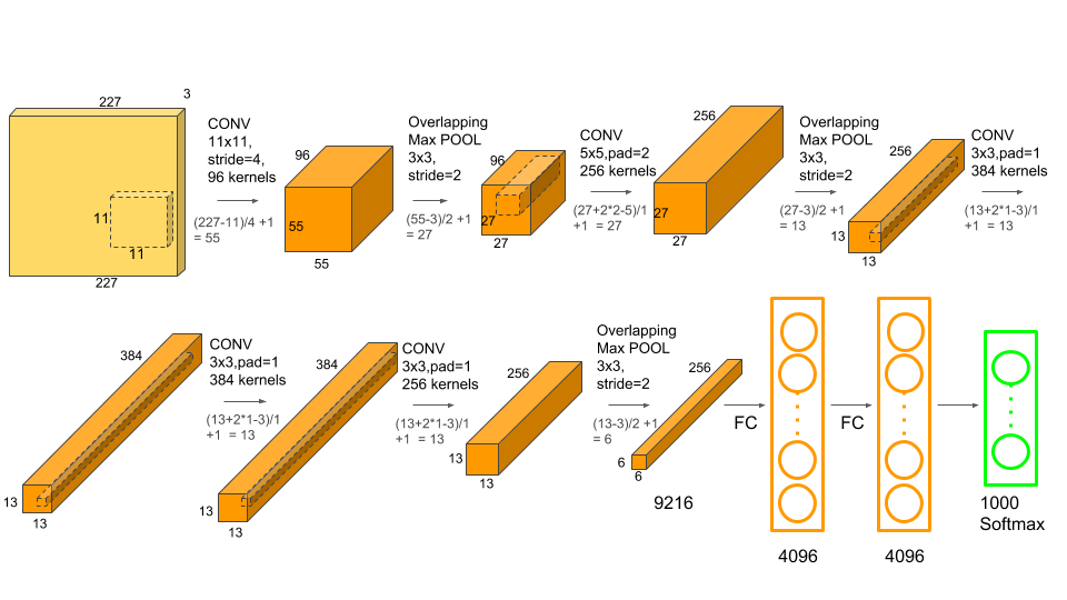 In the original AlexNet with convolution layers, max pooling layers, and fully connected layers, the total number of weight parameters is 62 million, and the activation map contains 195 million numbers in back-propagation with a batch size of 128. This adds up to 1.1 GB with single precision for each iteration. See [3][4] for detailed computation of memory size.
In 2012 when AlexNet was published [5], the state-of-art GPU had only 3 GB memory, which was not enough to store such a complex neural network model. So the authors of AlexNet ingeniously divided the model on 2 GPUs instead 1 GPU. These 2 GPUs mostly run in parallel and communicate only in certain layers, as shown in the figure below.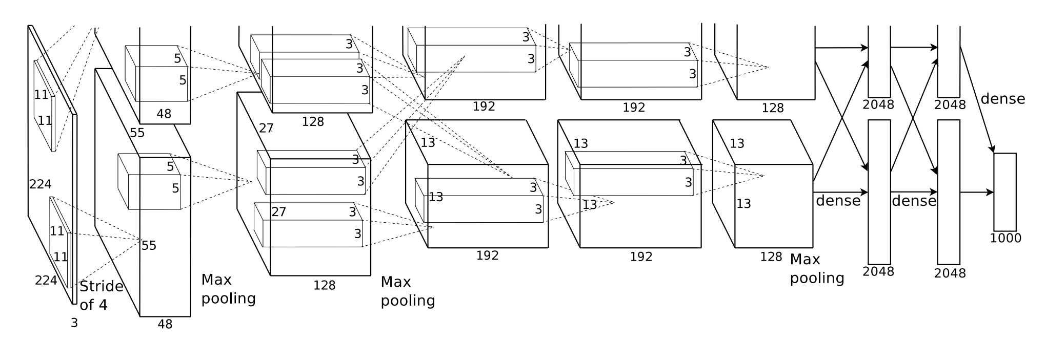
Scale up to more devices
In the same year as AlexNet, Google published DistBelief [6], a distributed framework that can use computing clusters with thousands of devices for model training.
Similar to AlexNet, DistBelief enables model parallelism and partitions the model across different devices through network communication or within the same device through multithreading. The difference is that DistBelief uses a large number of CPU cores, rather than 2 GPUs as in AlexNet, making the coordination and communication across devices more complicated. As shown the figure above, the network overhead starts to dominate as the number of devices increases, especially for less complex models. Models with more parameters (red lines) benefit more from the use of additional devices.
Model parallelism and Data parallelism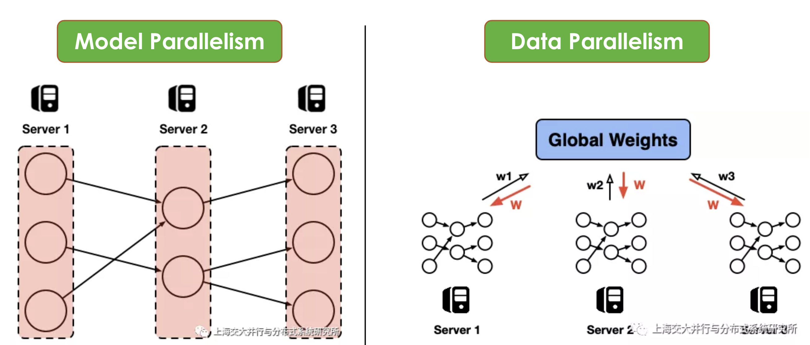
In addition to model parallelism, DistBelief also supports data parallelism. Similar to MapReduce, in DistBelief framework, data is partitioned on multiple servers, and each server runs their own computing in parallel. As shown in the right diagram above [7], assuming we are training a neutral net, each server holds a subset of the training data and a copy of the model itself. In each iteration, each server pulls the latest global weights \(w\) form a central server (blue box), computes the gradient \(\Delta w\) using its local data subset, and pushes the gradient back to the central server.
Each server updates the gradient in parallel (map), and the central server aggregates all updated gradients as the end of each iteration (reduce).
Parameter server in data parallelism
Figures in this session are from ref. [8].
The central server that stores model parameters is called a “Parameter Server”. It is commonly implemented as a key-value store, although there are other feasible implementations. When there are millions or billions of parameters or when there are a lot of workers in the cluster, a single parameter server may not suffice because of network bandwidth bottleneck between workers and the parameter server. To scale up for a large number of parameters, parameters can be sharded across multiple server nodes, and each parameter server stores only part of parameters. This is called “sharded key-value store” [9].
Server nodes communicate with each other to replicate and migrate parameters for scaling and reliability. A server manager coordinates all server nodes to maintain consistency.
The keys index the model parameters and the values are the parameter values of a model. For example, when we are training a linear regression model:
\(y = w_1*x_1 + w_2*x_2 + .. + w_N * x_N\)
The key-value store could look like
\(\{w_1: 0.2, w_2: 0.01, … w_N: 0\} \)
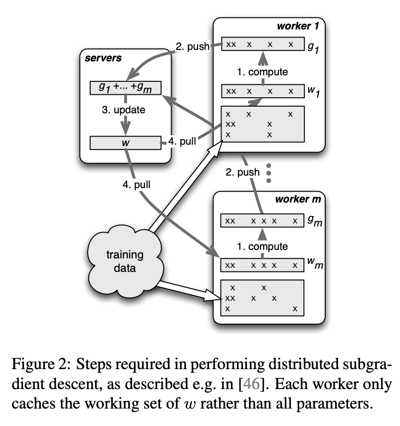
Each worker essentially pulls a weight vector from the parameter server with corresponding weight values \([0.2, 0.01, …0]\) and pushes the updated vector back to the parameter server. The parameter server then aggregates all the subgradients.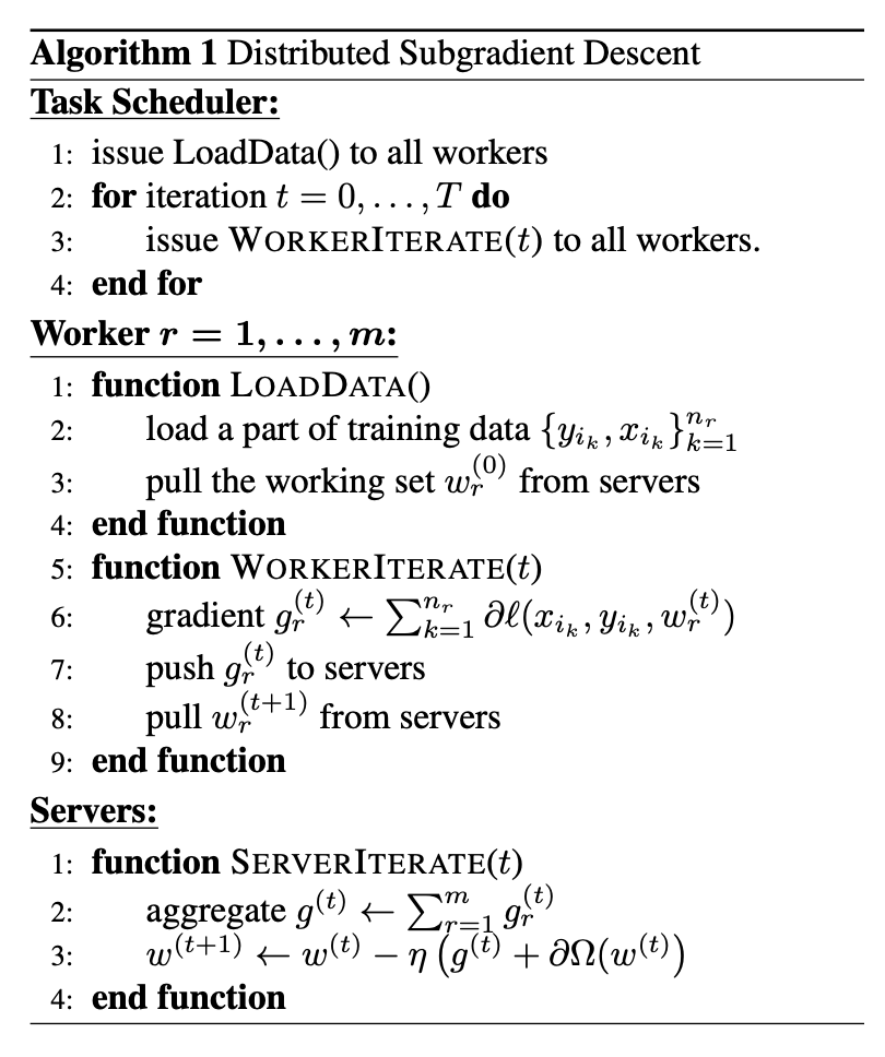
It is worth emphasizing that when data are partitioned in many workers, parameters on each data subset can be sparse as shown in the following diagram. The vectors passing between workers and the parameter server are also sparse, essentially reducing the model size on each worker and network communication cost.
 As more workers are used, each worker processes fewer parameters.
Synchronous and Asynchronous data parallelism
As described in the algorithm above, the parameter server aggregates updated weights from all workers. As different workers may have different computation time, the whole process could be blocked by the slowest machine. This is illustrated by the diagram below [10]. In this example, at the beginning of each iteration, 3 worker machines pull the latest global weight \(w\) from the parameter server, update local weights \(w^1, w^2, w^2\). When machine 1 and 3 finish computing, machine 2 is still running. The parameter server can only start to aggregate and compute global weight after receiving updated weights from all machines.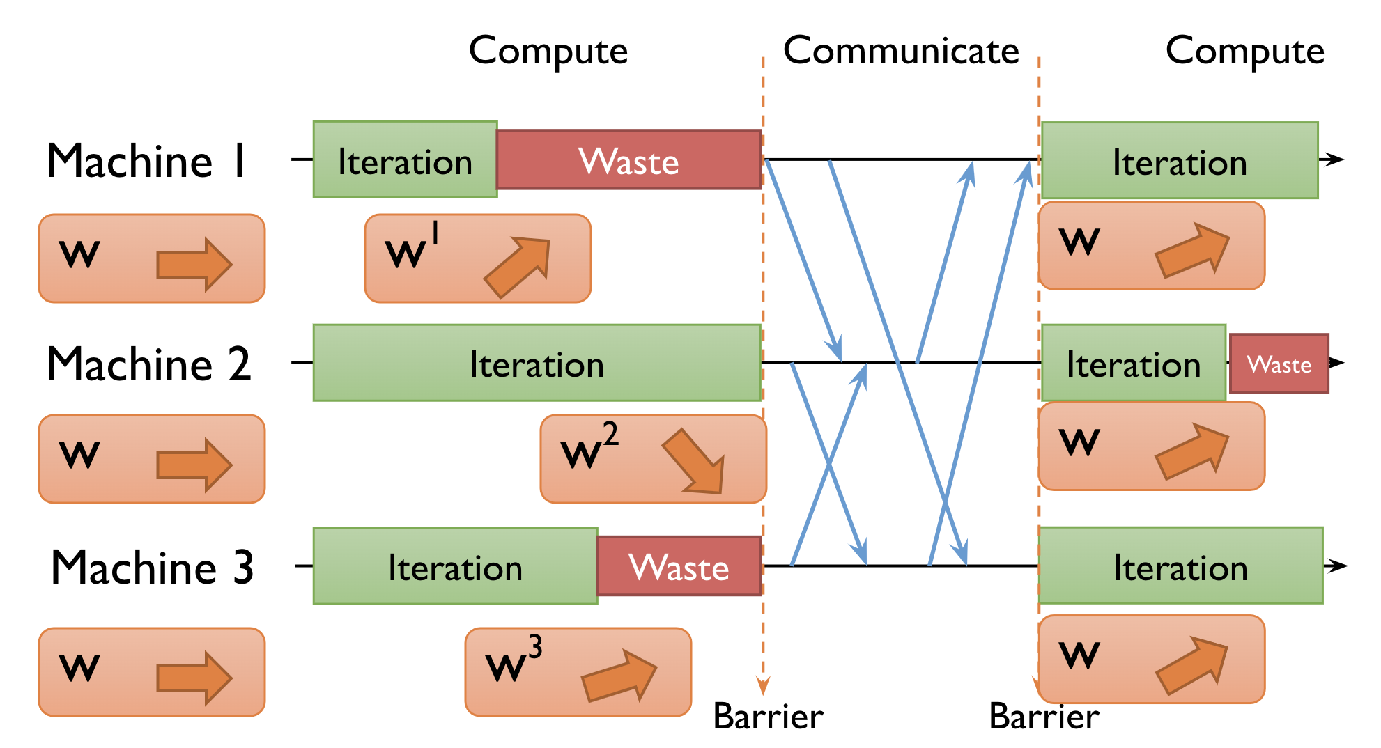
This is synchronous data parallelism. In DistBelief, it is called “Sandblaster L-BFGS” (the right diagram below), in which a single “coordinator” sends small messages to replicas and the parameter server to orchestrate batch optimization and synchronize weight update in each iteration. This execution mode fits naturally in the MapReduce paradigm. The major drawback of synchronous data parallelism is the waiting time (waste) on worker machines. Alternatively, we could allow workers to pull global weights from the parameter server as soon as they finish one iteration without waiting for all other workers. This mode is called asynchronous data parallelism. In DistBelief, it is called “Downpour SGD” (the left diagram above). As shown in the diagram below, each machine is constantly pulling and pushing parameters without waiting for other machines.
There are a few advantages of computing asynchronously. First, we are making the most of the computing capacity of worker machines without waiting time; Second, the partially updated and thus slightly outdated weight could add more stochasticity during training.
The asynchronous pattern however could also cause slow convergence and poor model stability due to stale parameters. In particular, the running iterations for each machine can be vastly different. In practice, we need to balance system efficiency and algorithm convergence.
What now?
It’s been 8 years since AlexNet and DistBelief were published, and study in distributed model training keeps developing. Here are a few recent trends in the field:
- Data parallelism is more commonly used than model parallelism. Data parallelism is quite straightforward to set up, whiles model parallelism usually requires delicate design of device connection and model partition.
- Parameter server is widely used in data parallelism.
- Asynchronous execution has been largely replaced by synchronous execution. This is mostly due to concerns about model stability and convergence. The “slowest machine” issue in synchronous execution can be mitigated by dropping slow machines after timeout to make sure the whole system is not delayed for too long.
- Combine data and model parallelism in pipeline parallelism. See PipeDream in ref [11] for more information.
- Decentralize parameter server. In the original design, there was a central parameter server that coordinated all workers. This could cause network communication bottleneck and slow down the system. Smart server topology aims to solve this problem, see the session below.
AllReduce
So far, we have discussed the benefit of distributing model training process on multiple machines. However, there is no free lunch with more computing power. As mentioned in the previous session, more machines do not necessarily accelerate the training process. With more machines in the network, the communication cost could quickly exceed the added computation benefit.
Classical parameter server
This is especially true when we have a central parameter server. In the following example, say we have 4 machines (e.g. GPU). Each machine stores their own copy of 4 parameters: 1, 2, 3, 4 with different versions a, b, c, d [10].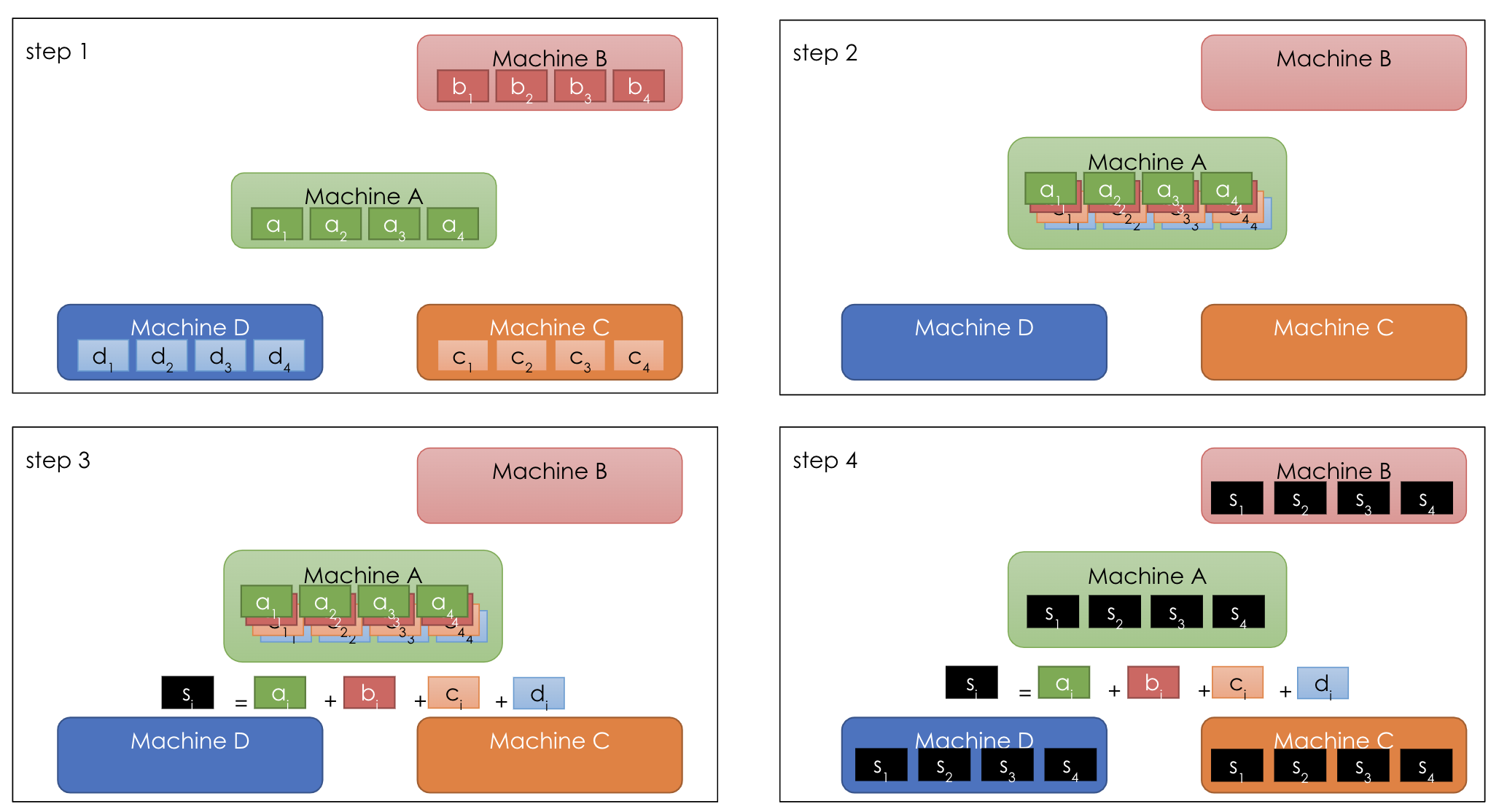 In the classical central parameter server paradigm, one machine (say machine A) does the aggregation jobs (reduce in MapReduce) while all other machines send different versions of parameters to A at step 2. At step 3, machine A aggregates of all versions for each parameter: \(s_i = a_i + b_i + c_i + d_i\). We could think \(a\) as the global weight, and \(b, c, d\) as the updated weights from each worker machine.
After machine A completes all aggregation, at step 4 it broadcasts results to all other machines. This could be viewed as each worker pulls the latest global weight from a central parameter server.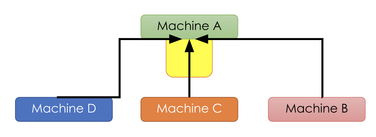 With this paradigm [10], the bandwidth required by machine A is \((P-1)*N\) where \(P\) is the number of machines and \(N\) is the total number of parameters. The bandwidth for machine A increases as we are adding more machines or having more parameters.
AllReduce
Instead of having a single machine to perform the aggregation task, we can distribute the aggregation task on all machines.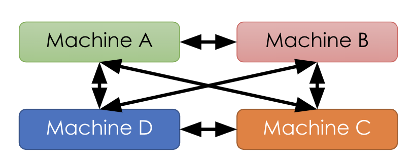 Let’s say, each machine aggregates a few parameters. In the diagram below, machine A aggregates different versions of parameter 1, machine B – parameter 2, and so on.
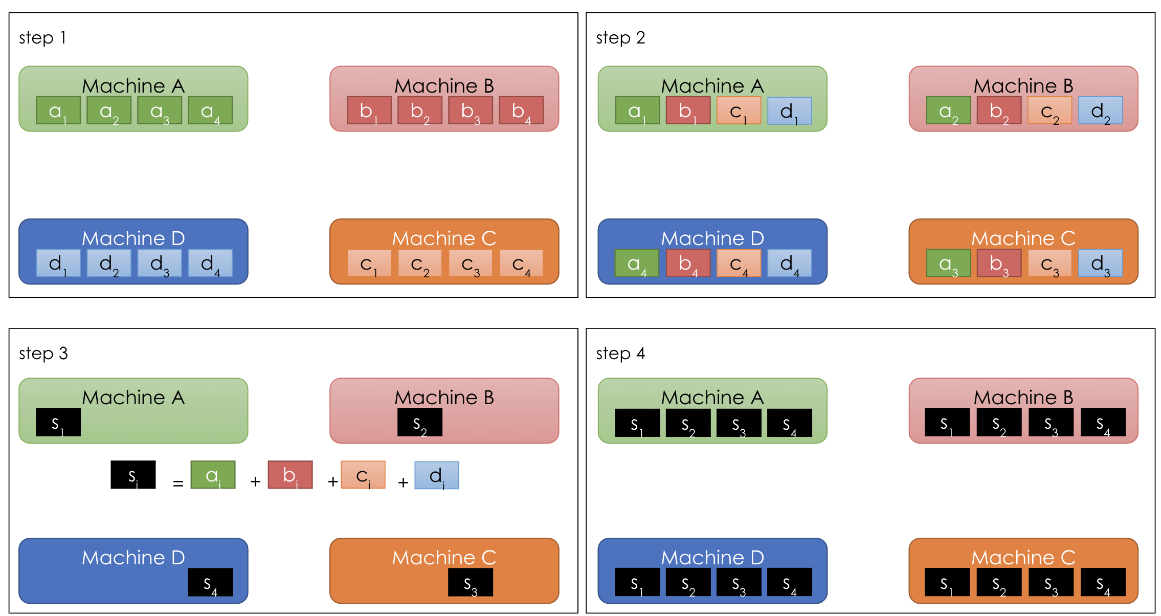
In the aggregation step 2, each machine sends its version of all parameters to all other machines; in the broadcast step 4, each machine sends its aggregated result to all other machines. This results in a bandwidth of \((P-1)*N/P \) for all machines, which is smaller than the one in parameter server \((P-1)*N\).
Ring AllReduce
A even more efficient network topology is Ring AllReduce. In this paradigm [10], all machines are set up in a ring. Similar to AllReduce, each machine performs the aggregation task on a subset of parameters: machine A – parameter 1, machine B – parameter 2, etc. Different from AllReduce, instead of sending its version of parameters to all other machines, each machine sends its version of parameters to the next one.
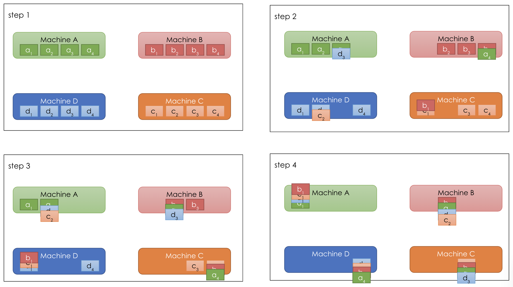 As shown in the diagram above [10], step 1: all machines start with their own copies of all 4 parameters 1,2,3,4; step 2: machine B sends parameter \(b_1\) to machine C, C sends \(c_2\) to D, D sends \(d_3\) to A, and A sends \(a_4\) to B; step 3 and step 4, similar to step 2. And the end of step 4, each machine has the full version of a subset of parameters: machine A has all four versions (a,b,c,d) of parameter 1 and aggregates them.
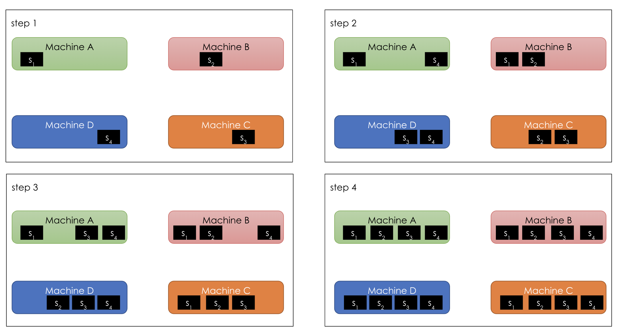 In the broadcast step above, each machine sends its aggregated results to the next machine: step 2: machine A sends \(s_1\) to B, B sends \(s_2\) to C, C sends \(s_3\) to D, D sends \(s_4\) to A. At the end of step 4, each machine has the aggregated form for all parameters.
At each round, we have a constant bandwidth of \(N\) that does not depend on the total number of machines \(P\), thus more scalable.
The limiting factor in Ring AllReduce is the number of rounds of communication, which equals to \(P-1\). As there are more machines, it may take longer for each cycle.
Tree AllReduce
Another AllReduce topology is tree structure.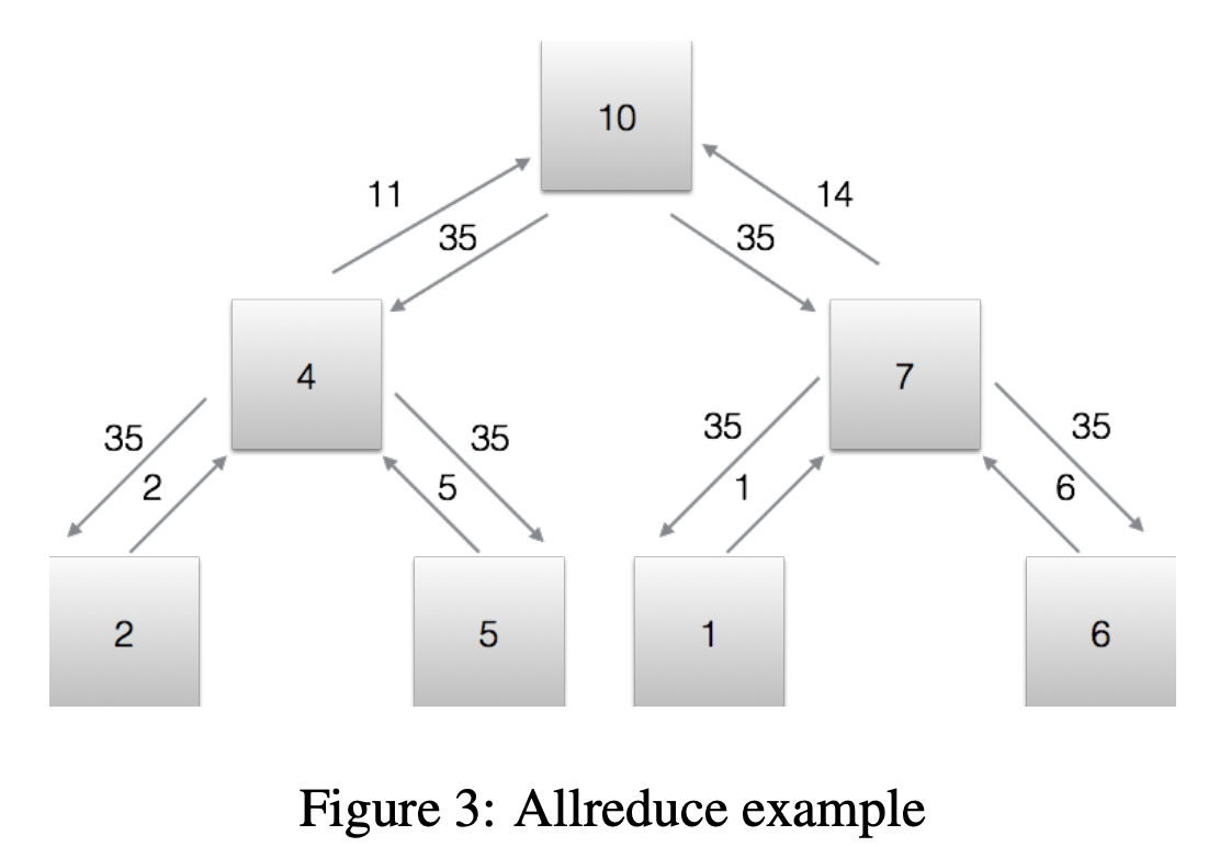
Each machine node holds a subset of data and computes some values (gradient) on it. Those values are passed up the tree and aggregated, until a global aggregate value is calculated in the root node. The global value is then passed down to all other nodes.
This tree-based AllReduce algorithm is the backbone of distributed XGBoost [13], called RABIT [14].
Use parameter server in your project
As machine learning practitioners, we do not need to reinvent the wheel and implement a parameter server from scratch. There are a lot of open-source and commercial solutions we can use directly to enable distributed model training. Two examples are shown below:
Distributed XGBoost
As discussed above, XGBoost uses the RABIT algorithm to distribute gradient boosted tree model [13-15].
Distributed Tensorflow
If you are using Tensorflow already, it is very easy to set up distributed model training using tf.distribute.Strategy.
See the official documentation for more details [16].
Takeaways
Distributed model training enables us to train bigger models with more data for better performance. From MapReduce, to Spark, to parameter server and AllReduce, the development of distributed model training highlights fruitful collaboration between machine learning and systems (MLSys).
References
cover image: https://commons.wikimedia.org/wiki/File:BalticServers_data_center.jpg
[1] https://en.wikipedia.org/wiki/Server_(computing)
[2] https://www.learnopencv.com/understanding-alexnet/
[3] https://www.learnopencv.com/number-of-parameters-and-tensor-sizes-in-convolutional-neural-network/
[4] https://medium.com/syncedreview/how-to-train-a-very-large-and-deep-model-on-one-gpu-7b7edfe2d072
[5] https://papers.nips.cc/paper/4824-imagenet-classification-with-deep-convolutional-neural-networks.pdf
[6] https://static.googleusercontent.com/media/research.google.com/en//archive/large_deep_networks_nips2012.pdf
[7] https://mp.weixin.qq.com/s/IQbBD_RxbeecrlPUiKcLjQ
[8] https://www.cs.cmu.edu/~muli/file/parameter_server_osdi14.pdf
[9] https://youtu.be/rnZmdmlR-2M
[10] PPT https://ucbrise.github.io/cs294-ai-sys-fa19/
[11] https://cs.stanford.edu/~matei/papers/2019/sosp_pipedream.pdf
[12] https://andrew.gibiansky.com/blog/machine-learning/baidu-allreduce/
[13] https://www.kdd.org/kdd2016/papers/files/rfp0697-chenAemb.pdf
[14] https://pdfs.semanticscholar.org/cc42/7b070f214ad11f4b8e7e4e0f0a5bfa9d55bf.pdf
[15] https://github.com/dmlc/xgboost
[16] https://www.tensorflow.org/guide/distributed_training