
Whenever we see the word “optimization”, the first question to ask is “what is to be optimized?” Defining an optimization goal that is meaningful and approachable is the starting point in function fitting. In this post, I will discuss goal setting for function fitting in regression.
This is No.3 post in the Connect the Dots series. See full table of contents.
In the case of a supervised learning problem, the goal essentially contains 2 parts:
- find a fitting function to minimize the objective function on training data
- select a fitting function to minimize the prediction error on testing data (the ultimate goal)
Notice that I use 2 different verbs here: find and select, which correspond to model training and model selection, respectively.
Let’s talk about model training first:
Goal: find a fitting function to minimize the overall objective function on the training data
\(Obj(f, X_{train}, y_{train}) = L(f(X_{train}), y_{train})) + J(f) \tag{1}\)
First, let’s look at the first element which captures the total prediction error on the training data \(L(f(X_{train}), y_{train})\). For simplicity, I will omit “train” in the subscript.
\(L(f(X), y) = \sum_{i=1}^{N} l(f(x_i), y_i) \tag{2} \)
Input \(X = (X_1, X_2, …, X_p)^T, X \in R^{N \times p}, x_i \in R^p\). In regression, output \(y_i \in R \); in classification, output \(y_i \in {1,2,…k} \) and \(k\) represents discrete class labels. In this post, I only discuss the regression problem, and in the next post, I will focus on the classification problem.
\(L\) is an aggregation of \(l\) over all data points, and it is sometimes averaged by the number of points \(N\) to represent the mean prediction error.
Our goal is to minimize \(L\) in Equation 2.
Table of Contents
A simple linear regression
Let’s start with a simple case \(p = 1, \beta_0 = 0, N=2\). Notice that \(N >= p+1\) in order to have a unique solution in the linear function. The 2 data points are denoted by \((x_1,y_1), (x_2, y_2)\) and 2 parameters by \(\beta_0, \beta_1\). All values are real numbers \(R\).
\(\hat y_1 = \beta_1 x_1 \tag{3.1}\)
\(\hat y_2 = \beta_1 x_2 \tag{3.2} \)
The total loss function to be optimized is \(L(f(X), y) = \sum_{i=1}^{N} l(\hat y_i, y_i) \)
A commonly used loss function is squared error:
\(l(\hat y_i, y_i)= (y_i – \hat y_i )^2 \tag{4} \)
Thus \(L\) can be written as:
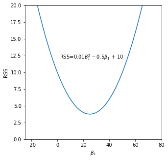
\(L = (y_1 – \beta_1 x_1)^2 + (y_2 – \beta_1 x_2)^2 = (x_1^2 + x_2^2) \beta_1^2 – 2(x_1y_1 + x_2y_2)\beta_1 + (y_1^2 + y_2^2) \tag{5} \)
This is a univariate quadratic function on \(\beta_1\). Equation 5 has the format of \(y = ax^2 + bx + c\), and here \(x\) is \(\beta_1\), and \(a \) is \((x_1^2 + x_2^2)\), which is non-negative. So the parabola will look something like the following diagram with a global minimum value:
We can compute the derivative of Equation 5 on \(\beta_1\) and set it as \(0\) to get the optimal value of \(\hat \beta_1\) for a minimum \(L\).
\(\frac {\partial L}{\partial \beta_1} = 2(x_1^2 + x_2^2) \beta_1 – 2(x_1y_1 + x_2y_2) = 0 \tag{6}\)
Solving Equation 6, we get
\(\hat \beta_1 = \frac {x_1y_1 + x_2y_2} { x_1^2 + x_2^2 } \tag{7.1} \)
which is the same as
\(\hat \beta_1 = \frac {Cov(X,y)} {Var(X)} \tag{7.2} \)
Linear regression model
Now let’s extend to the general format of linear regression model with input \(X = (X_1, X_2, …, X_p)^T, X \in R^{N \times p}\).
$$\begin{bmatrix}\hat y_1\\ …\\ \hat y_i\\ … \\ \hat y_N\end{bmatrix} = \beta_0\begin{bmatrix}1\\ …\\ 1 \\ … \\1\end{bmatrix} + \beta_1 \begin{bmatrix}(x_1)_1\\ …\\ (x_i)_1\\ … \\(x_N)_1\end{bmatrix} + … + \beta_j \begin{bmatrix}(x_1)_j\\ …\\ ( x_i)_j \\ … \\(x_N)_j\end{bmatrix} + … + \beta_p \begin{bmatrix}(x_1)_p\\ …\\ ( x_i)_p \\ … \\(x_N)_p\end{bmatrix} \tag{8} $$
In the matrix format, Equation 8 can be written as:
$$\hat y =\textbf{X}\beta \tag{9} $$
$$ \beta = [\beta_0, \beta_1, …, \beta_p ]^T \tag {10} $$
where \(\textbf{X} \in R^{N \times (p+1)} \) with a \(\textbf{1}\) in the first position of \(\beta_0\). \(y \in R^{N \times 1}\), and \(\beta \in R^{(p+1) \times 1} \).
Using the squared-error loss function, the matrix format of total loss \(L\) is:
\(L(\hat y, y) = (y – \textbf{X}\beta)^T(y – \textbf{X}\beta) \tag{11} \)
Here \(L \) is also called Residual Sum of Squares (RSS), which is closed related to mean squared error (MSE). \(MSE = \frac {RSS}{N} \). RSS has parameters \(\beta\) and we can write the loss function as \(RSS(\beta)\).
\(RSS(\beta) = (y – \textbf{X}\beta)^T(y – \textbf{X}\beta) \tag{12.1} \)
\(RSS(\beta) \\ = (y – \textbf{X}\beta)^T(y – \textbf{X}\beta) \\ = y^Ty – \beta^T \textbf{X}^Ty -y^T \textbf{X}\beta – + \beta^T \textbf{X}^T \textbf{X}\beta \\ = y^Ty – 2\beta^T \textbf{X}^Ty + \beta^T \textbf{X}^T \textbf{X}\beta \tag{12.2} \)
Notice that \(\beta^T \textbf{X}^Ty \) and \(y^T \textbf{X}\beta \) are both scalers and the transpose of a scaler is itself: \(\beta^T \textbf{X}^Ty = (\beta^T \textbf{X}^Ty)^T = y^T \textbf{X}\beta \).
Similar to Equation 5, Equation 12.2 is also a quadratic function on \(\beta\) with \(\beta^T \textbf{X}^T \textbf{X}\beta \). To find the \(\hat \beta \) that minimizes \(RSS\), we can take the derivative of Equation 12.2 with respect to \(\beta\) and get the following equation:
\(\frac {\partial RSS(\beta)} {\partial \beta} = -2 \textbf{X}^Ty + 2 \textbf{X}^T \textbf{X}\hat \beta = 0 \tag {13} \)
Solving Equation 13,
\(\textbf{X}^T \textbf{X}\hat \beta = \textbf{X}^Ty \tag {14.1} \)
\(\hat \beta = ( \textbf{X}^T \textbf{X}) ^ {-1} \textbf{X}^Ty \tag {14.2} \)
Computing the best \(\hat \beta\) analytically is possible because the squared-error loss function is differentiable.
The derivation of \(\hat \beta\) only requires the function to have a linear format, but does not make any assumptions on the data. As discussed in the previous post, more assumptions are required when we need to make inference of the parameters.
Squared error and mean
An interesting feature of \(\hat \beta\) is that the function goes through the mean, \((\bar {\textbf{X}} , \bar y) \), i.e. \(\bar {\textbf{X}} \hat \beta = \bar y \).
\(\bar {\textbf{X}} = \frac {\textbf{X}}{N} \tag {15.1}\)
\(\bar y = \frac {y}{N} \tag {15.2}\)
\(\bar {\textbf{X}} \hat \beta \\ = \bar{\textbf{X}} (\textbf{X}^T \textbf{X}) ^ {-1} \textbf{X}^Ty) \\ = \frac {\textbf{X}(\textbf{X}^T \textbf{X}) ^ {-1} \textbf{X}^Ty}{N} \\ = \frac {\textbf{X} \textbf{X}^{-1}(\textbf{X}^T)^{-1}\textbf{X}^Ty} {N} \\ = \frac {y}{N} \\ = \bar y \tag{16} \)
In fact, when the loss function is squared error, the best prediction of \(y\) at any point \(\textbf{X} = x\) is the conditional mean.
But mean has an infamous drawback: it is very sensitive to outliers. How can we mitigate the effect of outliers?
Absolute error and median
Similar to the squared error, the absolute-error loss function also considers the difference between each \(\hat y_i \) and \(y_i\).
\(l(\hat y_i, y_i) = |y_i – x_i\beta| \tag {17} \)
\(L(\hat y, y) =\sum_{i=1}^{N}|y_i – x_i\beta| \tag {18}\)
Similar to Equation 12, we can derive \(L\) with respect to \(\beta\).
The derivative of absolute value can be written as:
$$ |f(x)| = f(x)^2 $$
\(\frac {\partial L(\hat y, y) }{\partial \beta} =\sum_{i=1}^{N} sign(y_i – x_i\beta) \tag {19.1}\)
\(sign(y_i – x_i\beta) =\begin{cases}
1, & y_i > x_i\beta \\
-1, & y_i < x_i\beta \\ 0, & y_i = x_i\beta \\
\end{cases} \tag {19.2}\)
The derivative is 0 when there are same number of positive and negative terms in \(y_i – x_i\beta\). This intuitively means \(\beta \) should be the median of \((X,y)\). Median, different from mean, is less sensitive to outliers, and thus more robust.
Loss function for linear regression
We have discussed squared error and absolute error as the loss function for regression. Both of them are differentiable, which means we can calculate the best parameters analytically.
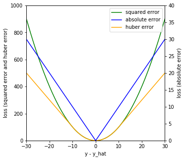
Squared-error loss (green curve) places more emphasis on observations with large margin \(|y_i – \hat y_i|\), and changes smoothly near loss 0. Absolute-error loss (blue curve) is more robust with large margin. Huber-error loss (yellow curve) combines the properties of both squared error and absolute error with a threshold \(\delta \). Below the threshold, it uses the squared-error loss, and above the threshold, it uses the absolute-error loss.
Loss function for other regression models
So far, I focused on the linear regression model, which enjoys the benefit of clear mathematical format and analytical solutions. It lays the foundation for the generalized linear model.
Other regression models such as the tree-based model and ensembles, do not use the same linear function as in linear regression. I will discuss tree-based models in details in later posts.
Here, I want to emphasize the choice of loss function, regardless of which regression model we are using. It is important to choose a loss function \(l\) that is differentiable with respect to the fitting function \(f\), so that we can compute the gradient which allows us to greedily and iteratively approach the optimization goal. If the loss function \(l\) is not differentiable, we are essentially facing a black box fitting function, which is very challenging to optimize.
Take home message
First, in linear regression, when using squared error to minimize the loss function, the best \(\hat \beta\) is the mean of training data; when using absolute error, the best \(\hat \beta\) is the median. Second, different goals (loss function) can generate different predictions. Third, it is important to choose a differentiable loss function.
Demo code can be found on my Github.
References
- https://web.stanford.edu/~mrosenfe/soc_meth_proj3/matrix_OLS_NYU_notes.pdf
- https://stats.stackexchange.com/questions/92180/expected-prediction-error-derivation
- https://stats.stackexchange.com/questions/34613/l1-regression-estimates-median-whereas-l2-regression-estimates-mean
- http://web.uvic.ca/~dgiles/blog/median2.pdf
- https://web.stanford.edu/~hastie/ElemStatLearn/