In the previous post, I discussed the function fitting view of supervised learning. It is theoretically impossible to find the best fitting function from an infinite search space. In this post, I will discuss how we can restrict the search space in function fitting with assumptions.
This is No.2 post in the Connect the Dots series. See table of contents.
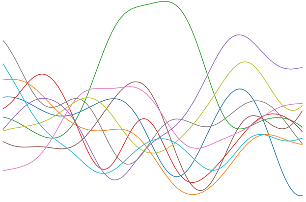
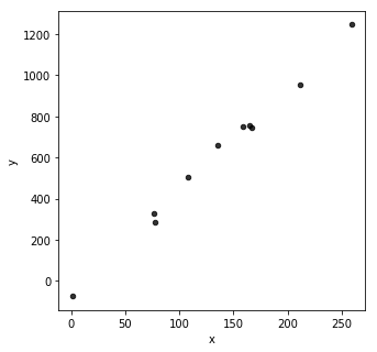
In the following example, we do not know for sure what the fitting function \(f\) should look like. We may guess the function is linear, polynomial, or non-linear, but our guess is as good as randomly drawing some lines connecting all the points. There are infinite number of functions in the space, and it is in theory impossible to iterate all of them to find the best one.
A lazy and naive way to predict unseen data is to use the “proximity rule” with the algorithm k nearest neighbor (KNN). For a new input data point \(x^{\prime}\) in \(X_{test}\), our assumption is that the predicted output \(\hat y_{test}\) can be represented by the \(k\) nearest neighbors in the training data \(X_{train}\), and we use the aggregated training output as the predicted output:
\(\hat y_{test}( x_i^{\prime}) = \frac {1} {k} \sum_{x_i \in N_k(x)} y_i \)
Here, \(N_k(x) \) is the neighborhood of \(x_i^{\prime}\) defined by the \(k\) nearest training points \(x_i\).
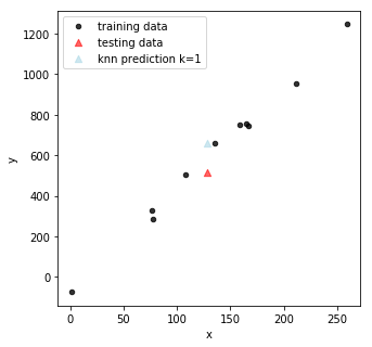
In this figure, the red triangle is the real testing data point and the light blue triangle is the KNN prediction with \(k = 1\): the prediction takes the nearest training data and assign \(y_{train}\) to the testing data.
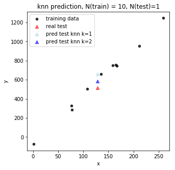
As we increase \(k = 2 \), we can see the prediction (darker blue triangle) gets closer to the real output (red triangle).
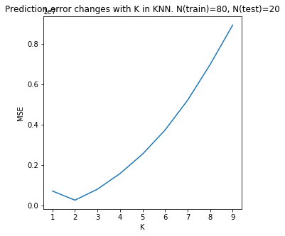
We can play with different \(k\) values and select the one with lowest prediction error (mean square error). Prediction error is related to bias variance trade-off: at low \(k\), the prediction heavily depends on a small local neighborhood with small number of training data, thus with low bias but high variance; at high \(k\), the prediction is made from larger number of training data set and becomes more global, thus with low variance but high bias.
KNN is also applicable to discrete output (classification problem). In the following example with 2-D input, we use \(k=1\) to make prediction for testing data.
 As shown in the bottom right figure, of the 20 testing data, 2 are misclassified (red) based on 100 training data. The prediction error of classification is usually not computed by mean squared error, but by different loss functions (summarized in later posts).
From a fitting function perspective, KNN builds a function \(f\) which performs pair-wise computation between all \(X_{train}\) and \(X_{test}\). Therefore, KNN is computationally expensive, particularly for large data. With \(n\) training data of \(p\) dimension and \(m\) new testing data, we have to compute the similarity matrix \(m \times n\), and then get the top \(k\) smallest distance for each testing data. The time complexity of KNN is O(np + nk).
To better restrict the search space for fitting functions and to reduce computation cost, most of the time, we make some assumptions about the data and functions.
A commonly used fitting function is Ordinary Least Square (OLS) which has 5 assumptions to guarantee that the OLS estimator is BLUE (best linear unbiased estimator), introduced in most statistics 101 courses. In practice, when we apply linear regression fitting, we need to define and assume the format of the linear function (linear, polynomial, or piece-wise), but we do not need to make any assumptions to compute the parameters that minimize the total loss function, shown in the next post.
These assumptions are critical, however, if we would like to make any inferences about the real parameter values. Say we want to understand if output \(y\) is correlated with an input \(X_1\). We can always use OLS to compute the parameter \(\hat \beta_1\). But how confident are we about the estimated parameter value? Is the correlation significant?
It is worth noticing that function fitting and statistical inference are related yet distinct topics. The latter usually has more strict assumptions.
- linear in parameters
- can be non-linear on the input
- \(y = \beta_0 + \beta_1 x + \varepsilon\)
- \(y = \beta_0 + \beta_1 x + \beta_2 x^2+ \varepsilon\)
- \(y = \beta_0 + \beta_1 log(x)+ \varepsilon\)
- counterexample: non-linear in parameters \(y = \beta_0 + \beta_1 ^ 2 x \)
- each data point is randomly and independently sampled
- \((x_i, y_i) \sim i.i.d. \)
- The error term \(\varepsilon\) should also be independent and random
- The number of input (N) should be larger than the number of parameters of each input (p): N>=p. Otherwise, the resulting parameters will not be unique (discussed in later post).
- 0 conditional mean of error
- \(E(\varepsilon|X) = 0 \), which is equivalent to \(cov(x_i, \varepsilon_i) = 0 \)
- error does not depend on the input
- no perfect collinearity in parameters
- counterexample
- \(X_1 = 2X_2\)
- \(y = \beta_1X_1 +\beta_2X_2 + \beta_3X_3\) can be written as \(y = \beta_1 (2X_2) +\beta_2X_2 + \beta_3X_3 = (2\beta_1 +\beta_2)X_2 + \beta_3X_3 = \beta_{12}X_2 + \beta_3X_3\)
- We may compute a unique \(\beta_{12}\), but cannot derive unique values for \(\beta_1\) and \(\beta_2\) as there are infinite solutions in \(\beta_{12} = 2 \beta_1+\beta_2 \)
- As a result, we cannot disentangle the effect of \(X_1\) and \(X_2\).
- counterexample
- homoskedastic error
- \(Var(\varepsilon|X) = \sigma^2 \)
- Error terms for each data point should be i.i.d., i.e. there is no autocorrelation between error terms \(Cov(\varepsilon_i \varepsilon_j | X) = 0\), for \(i \neq j\)
Linear function is one of the most basic supervised learning fitting functions, and is extremely powerful. I will discuss linear function in detail in the next post.
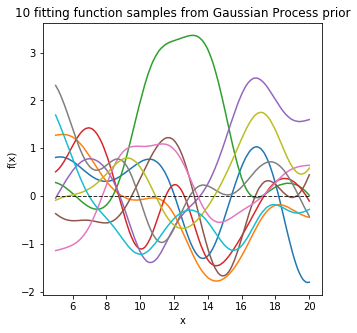
Another commonly used function is Gaussian Process (GP). GP makes assumptions of the prior distribution of fitting functions, and assumes any finite number of these functions have a joint Gaussian distribution. Say we have input data \(x_1, x_2, …,x_N\), and a GP assumes that \(p(f(x_1), f(x_2), …, f(x_N))\) is joint Gaussian.
For example, before we see any data, we can define a GP prior distribution of fitting functions for a 1-D input with mean of 0 as shown below.
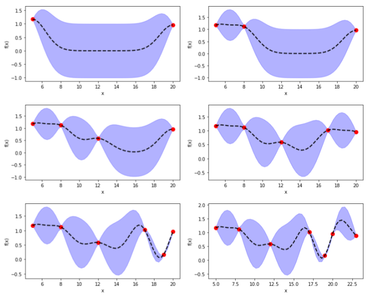
As we have more training data (red dots below), we can update the GP posterior distribution with the GP mean (dashed line) and standard deviation (purple area). As we can see, more training data will decrease variance for prediction.
GP has been widely applied in optimization of black-box functions. As will be discussed in later posts, quite a lot of supervised learning algorithms and fitting functions have a differentiable loss function and relay on gradient based approach for function optimization. However, in the case of gradient free functions, particularly if the objective function is highly convoluted and not directly differentiable, GP has great advantages and application such as Bayesian Optimization in hyperparameter tuning. I will discuss Gaussian Process in detail in later posts.
Take home message
Finding the best fitting function from an infinite function space is theoretically impossible. In order to practically find the “best” fitting function, we usually restrict the function space and make key assumptions about the data and the fitting function. Under these assumptions, we can optimize the fitting function with manageable computational complexity.
Demo code can be found on my Github.