In this very first post of the Connect the Dots series, I set up the supervised learning problem from a function fitting perspective and discuss the objective of function fitting.
This is No.1 post in the Connect the Dots series. See table of contents.
In a supervised learning problem, we have a bunch of input (also referred to as feature, independent variable, predictor) and the corresponding output (also referred to as label, target, response, dependent variable) as our observed and known training data. The goal is to fit a function (also referred to as “train a model”) and use it to predict output for unknown input.
We denote the input by \(X = (x_1, x_2, …, x_N)\), the output by \(y = (y_1, y_2, …, y_N) \), and the fitting function by \(f \). Each input \(x_i \in R^p \) has \(p\)-dimensions, and each output \(y_i\) can be either continuous values \(R\) in a regression problem, or discrete values such as \(\{0,1\}\) in binary classification. The training data \(D \) consists of pairs of input and output \(D = \{D_1, D_2, …, D_N\}, D_i = (x_i, y_i)\).
\(f \) takes \(X \) as input and calculates \(\hat y\) (pronounced as y hat) as the predicted output.
\(\hat y = f(X) \tag {1} \)
The difference between each predicted output and real output point is captured by loss function \(l \).
\(l(\hat y_i, y_i) = l(f(x_i), y_i) \tag {2} \)
The average loss over all data points is usually called cost function \(L \). Sometimes, people also use the term loss function to refer to cost function.
\(L(f(X), y) = \frac {\sum_{i=1}^N l(f(x_i), y_i)}{N} \tag {3} \)
The goal is to find a \(f \) which minimizes \(L\)
\(argmin_f L(f(X) , y) \tag {4} \)
Now the supervised learning problem is formulated as a function fitting problem. There are infinite number of functions in the problem space, as many as your imagination goes, and even beyond that!
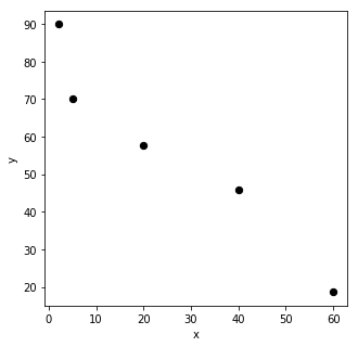
For example, we have 5 data points in our training data plotted as black dots. \(X\) is 1-D input and \(y\) is 1-D continuous output.
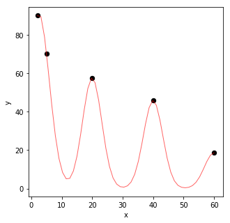
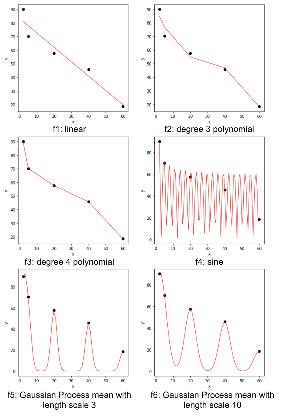
We have the freedom to draw whatever functions to fit the data. Let’s consider the following 6 choices of functions (red curves). As we can see, \(f_1 \) is a simple straight line, but we are not able to go through all points. \(f_2 \) concatenates several straight lines, and tries to go close to all points. \(f_3 \) goes through all the points. \(f_4 \) is a really wild one: it goes up and down with certain frequency and changing amplitude and also goes through all the points. \(f_5\) and \(f_6\) look similar, although \(f_6\) is smoother than \(f_5\).
The actual function I used to generate the data is \(f(x) = 60|e^{\frac {1}{x}} \times sin(x) | \), as shown by \(f_4 \).
Since our goal is to find a function \(f \) to minimize \(L\), if the function passes through all the data, the loss would be minimal (here it is 0). Can we then say \(f_3\) is better than \(f_1\)? How do we compare \(f_3 \) to \(f_4 \) given that they both have ideal minimal loss? Do we choose a simple function \(f_1 \) over other more complex functions? Do we choose a smooth function \(f_6\) over non-smooth function \(f_5\)?
More importantly, we would like to use the fitting function to predict unseen data. Say now we have new data \(X_{test} \) generated from the same population, the predicted \(\hat y_{test} \) is most likely not on the fitting function line except in \(f_4 \), because it is the function I used to generate both \(X_{train} \) and \(X_{test} \). Other fitting function may work perfectly on the training data (\(f_3, f_4, f_5, f_6\)), but not so well on the testing data.
In the end, the one and only golden standard for a good function is that it is able to predict unseen data as accurately as possible, in other words, minimize the error for unseen data.
Of course, what is “unseen” cannot be seen. So in theory, we cannot measure the performance of the function on “unseen” data. In practice, we split the whole seen data into training data and testing data, use the training data for function fitting, and use the testing data as the “unseen” data for function evaluation.
Here, we assume the real unseen data have the same characteristics as the seen data. This is not always the case: if our seen data is a biased sample from the whole population, or if the unseen data starts to deviate from the seen data as time goes by, the seen data may not well represent the real unseen data.
For simplicity, we assume the seen data is representative, and have the same distribution as the real unseen data. We redefine the goal of the problem as minimizing \(L\) for the “unseen” testing data (which in fact, is seen).
\(argmin_f L(f(X_{test}) , y_{test}| X_{train}, y_{train}) \tag {5} \)
The bad news is we cannot directly solve Equation (5) because \(f\) is fitted using the training data, not the testing data. The good news is training and testing data are from the same distribution, since we split the original seen data into these two. The difference between training and testing data thus originates from the variance of the data itself.
Let’s define Error as the following:
\(Error = L(f(X_{test}) , y_{test}) – L_{best} \tag {6.1} \)
\(Error = (L(f(X_{train}), y_{train}) – L_{best}) + (L(f(X_{test}) , y_{test}) – L(f(X_{train}), y_{train})) \tag {6.2}\)
Here, \(L_{best} \) denotes the loss in the best possible prediction function out there. It could be based on human performance. In a noise-free world, as in the first example, \(L_{best} = 0\). In practice, data is often noisy and \(L_{best} > 0\). We can treat \(L_{best} \) as a constant that is not affected by the data or the function. For simplicity, I omit \(L_{best}\).
The first element, called bias, represents how far the training data performs v.s the best possible one. The function fitting process can minimize this directly.
\(L(f(X_{train}), y_{train}) \tag {7}\)
The second element, called variance, represents how far the testing data performs v.s. the training data.
\(L(f(X_{test}) , y_{test}) – L(f(X_{train}), y_{train}) \tag {8} \)
Variance corresponds to the “generalization” of the fitting function. Our function may have very low bias, i.e. perform well on the training data, however, it may generalize badly on the testing data, thus high variance.
Variance is usually not directly solvable. In order to evaluate the performance of a function on “unseen” data, we usually use cross-validation to assess a fitting function after the training is done. In some cases, we may directly adjust and reduce variance by penalizing complex models. More complex models tend to better fit the training data and have lower bias, at the same time, the more the fitting function depends on the specific pattern in the training data in a complex model, the less well it generalizes. Therefore, we can add a penalty term to account for model complexity. Note that although penalty term is not exactly the same as variance, it captures the intrinsic difference of function performance on training and testing data. Cross-validation represents out-of-sample evaluation of a function, and penalty term (such as in Akaike information criterion) can be viewed as in-sample evaluation of a function. I will discuss more about function evaluation in later posts.
As shown in the example below, as we increase the degree of the polynomial fitting, the training mean squared error decreases while the testing mean squared error increases. The actual function I used to generate the data is \(y = 5 \times x – 3 + 10 \times N(5,3) \) with a Gaussian error.
| degree | training mean squared error | testing mean squared error |
|---|---|---|
| 1 | 786.83 | 867.83 |
| 2 | 785.29 | 873.93 |
| 3 | 785.28 | 874.16 |
In practice, during function fitting, we could add a penalty function \(J\) to \(L\), as shown in Equation (9) Objective function. Note that the penalty function depends only on the function of choice, not on the data directly. Although as we will see later, the function of choice is still decided based on the data.
\(Obj(f, X_{train}, y_{train})= L(f(X_{train}), y_{train}) + J(f) \tag {9}\)
The bias-variance trade off is ubiquitous in machine learning as whatever pattern we discover from the seen data may not be exactly the same in unseen data.
Take home message
Eventually, we want a generalizable fitting function that allows us to predict real unseen data accurately. We can do this by choosing the function that minimizes loss on “unseen” testing data.
\(argmin_f L(f(X_{test}) , y_{test}|X_{train}, y_{train}) \)
We use the training data to find the best possible \(f\) by optimizing the objective function which takes into consideration both loss and function complexity.
\(Obj(f, X_{train}, y_{train})= L(f(X_{train}), y_{train}) + J(f)\)
Demo code can be found on my Github.