Now what we have discussed unconstrained optimization problems in previous post, it is now time to come to the reality. In the real world, we often have limitations, such as the total budget, motion angles, and some arbitrary desirable range of values. Life would be so easy (and boring) without boundary and conditions. Adding constraints certainly makes optimization problems less easy, but more interesting.
This is No.10 post in the Connect the Dots series. See full table of contents.
Constrained optimization problems are defined with the objective function and the constraint functions:
$$ \min f(x) \tag {1} $$
$$ s.t. $$
\(h(x) = 0, h(x) = (h_1(x), h_2(x), … h_m(x))^T \in R^m \tag{2}\)
\(g(x) \leq 0, g(x) = (g_1(x), g_2(x), … g_n(x))^T \in R^n \tag{3}\)
Equation 2 represents equality constraints and equation 3 represents inequality constraints [3].
A set of points satisfying all constraints define the feasible region \(K\):
$$ K = \{x \in R^n | h(x) = 0, g(x) \leq 0 \} \tag{4} $$
The optimal point that minimizes the objective function is denoted as \(x^{*}\):
$$ x^{*} = argmin_{x \in K} f(x) \tag {5} $$
Equality constraint
Function values can be represented as contours on which the function values are the same across different input values. For example, when we only have one equality constraint function \(h_1(x)\), as shown in the following figure, the contours of objective function (blue circles) \(f(x)\) and equality constraint function (red curve) \(h_1(x)\) “barely” intersect, which means two functions are tangential [2].
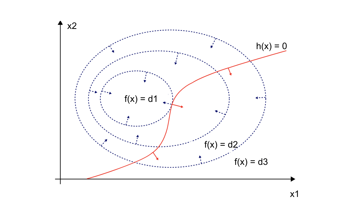
Geometrically, this means the gradients of \(f(x)\) (blue arrows) and \(h(x)\) (red arrows) are proportional to each other, with a multiplier \(\lambda \).
\(\nabla f(x) = \lambda \nabla h(x) \tag{6}\)
We can re-write the objective function from equation 1 and 2 as
$$ L(x, \lambda) = f(x) – \lambda h(x) \tag{7} $$
$$ \lambda h(x) = \sum_{i=1}^m \lambda_i h_i(x) \tag{8} $$
Note that in equation 7, \(h(x) = 0\). In practice, we could have \(h(x) = b\), while \(b\) is some constraint constant. We can write it as \(h(x) – b = 0\), and have
$$ L(x, \lambda) = f(x) -\sum_{i=1}^m \lambda_i (h_i(x) – b_i)\tag{9}$$
To minimize \(L\) in equation 9, we compute its first derivative:
$$ \nabla L = 0 \tag{10} $$
$$ \nabla L(x) \\= (\frac {\partial L}{\partial x_1}, \frac {\partial L}{\partial x_2} … \frac {\partial L}{\partial x_n}) \\ = \nabla f(x) – \lambda \nabla h(x) = 0 \tag{11} $$
$$ \nabla L(\lambda) \\ = \frac {\partial L}{\partial \lambda} \\= -( h(x) – b) = 0 \tag{12}$$
As we can tell, equation 12 represents constraint conditions, and equation 11 represents the proportional relationship between the gradients of the objective function and the constrained function, with the Lagrange multiplier:
\(\lambda = \nabla h(x) ^{-1} \nabla f(x) \tag{13} \)
What does \(\lambda\) mean? The minimum of \(L\):
\(L^{*} = argmin_{\lambda} f(x) – \lambda (h(x) – b) \tag{14} \)
When we treat the equality constraint \(b\) as a variable, \(L^{*}(b) \) [2], and we have:
\(\frac {\partial L^{*}}{\partial b} = \lambda \tag{15} \)
This means the minimum of \(L\) changes with \(b\) at a rate of \(\lambda\).
Inequality constraint
When we have inequality constrained conditions, things are a little bit more complicated.
In fact, inequality constrained conditions in equation 3 can be written as
\(g(x) = 0 \tag{3.1} \)
\(g(x) < 0 \tag{3.2} \)
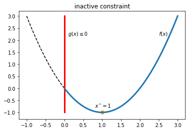
Let’s start with an example with \(x \in R\). \(f(x)\) is a quadratic function (black dashed curve), \(g(x) \leq 0 \) represents the region on the right side of the straight vertical line (red), and blue curve represents feasible region of \(f(x)\).
In the first scenario when the minimum \(x^* \) (orange dot) is on the right side (feasible region) of the vertical line, the constraint is inactive. We can treat the problem as an unconstrained optimization problem:
\(\nabla f(x) = 0 \tag{16} \)
In the second scenario where the minimum \(x^* \) is on the vertical line, and the minimum (orange dot) for \(f(x)\) is not in the feasible region (blue curve). The constraint is thus active.

As we can see from the figure above, at the red boundary, \(f(x)\) is not at its minimum, and there is a descent direction \(p\) at point \(x^*\) satisfying:
\(\nabla f(x^*) p < 0 \tag{17}\)
And since \(g(x^*) = 0\), any other \(x\) would have \(g(x) < 0\), this means \(x^*\) is the maximum point for \(g(x)\). For any descent direction \(p\) satisfying equation 17, \(p\) must have:
\(\nabla g(x^*) p \geq 0 \tag{18}\)
If \(\nabla g(x^*) p < 0\), \(x^*\) is not a stable local maximum for \(g(x)\).
Combing equation 17 and equation 18, we have
\(sign(\nabla f(x^*)) = – sign(\nabla g(x^*) ) \tag{19}\)
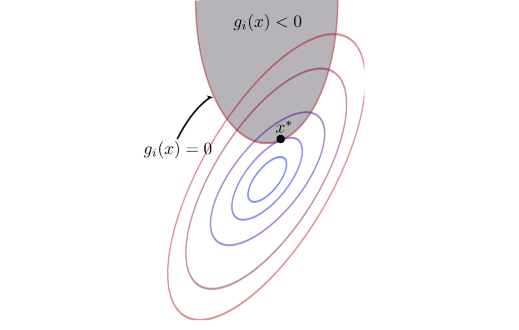
The relationship in equation 19 is well depicted in the following figure [5], using the contour plot. As we can see, at the boundary, the gradient of \(f(x)\) and \(g(x)\) are parallel.

\(\nabla f(x) = – \mu \nabla g(x) \tag{20}\)
\(\mu \geq 0 \tag{21}\)
We can generalize Lagrange multiplier in equation 9 to the inequality constraint problem. \(\mu\) is also called a KKT multiplier or dual variable [4].
$$ K(x, \mu) = f(x) + \mu g(x)\tag{22.1} $$
$$ \mu g(x) = 0 \tag{22.2}$$
$$ \mu \geq 0 \tag{22.3} $$
$$ g(x) \leq 0 \tag{22.4}$$
Equation 22 represents the 2 scenarios discussed
1. \(\mu = 0\), \(g(x) < 0\)
\(K(x) = f(x) \tag{23} \)
Equation 23 is an unconstrained problem.
2. \(\mu > 0\), \(g(x) = 0\)
\(K(x) = f(x) + \mu g(x) \tag{24} \)
Equation 24 is an equality constraint problem.
\(\nabla K(x) = \nabla f(x) + \mu \nabla g(x) = 0\)
\(\nabla K(\mu) = g(x) = 0 \)
Summary
Combining equation 9 and 22, we have
\(L(x, \lambda, \mu) = f(x) + \sum_{i=1}^m \lambda_i h_i(x) + \sum_{i=1}^m \mu_i g_i(x) \tag{25}\)
Note that there is no sign restriction for Lagrange multiplier \(\lambda\) and we can use either plus in equation 25, or minus in equation 9.
To minimize \(L\), we get its first derivative w.r.t. \(x, \lambda, \mu\).
Stationary:
\(\nabla L(x) = \nabla f(x) + \sum_{i=1}^m \lambda_i \nabla h_i(x) + \sum_{i=1}^m \mu_i \nabla g_i(x) = 0 \tag{26.1}\)
Equality :
\(h_i(x) = 0, i = 1,2,…m \tag{26.2}\)
Inequality:
also called complementary slackness condition
\(\mu_i g_i(x) = 0, i = 1,2,…n \tag{26.3}\)
\(\mu_i \geq 0 \tag{26.4}\)
\(g_i(x) \leq 0 \tag{26.5}\)
KKT condition provides analytic solutions to constrained optimization problems. In practice, analytic computation for stationary points can be difficult. As in unconstrained problem, we may use iterative approaches to compute a solution with feasible descent directions.
Last but not the least, there are 2 special types of optimization problems: linear optimization and quadratic optimization. They have simple mathematical format and are widely applied in real-world problems. Several approaches have been developed to tackle these 2 special optimization problems. See [3] for further reading.
References
[1] cover image: https://commons.wikimedia.org/wiki/File:Inequality_constraint_diagram.svg
[2] youtube: https://www.youtube.com/watch?v=m-G3K2GPmEQ
[3] Numerical Optimization, Jorge Nocedal, Stephen J. Wright
[4] https://github.com/wzhe06/Ad-papers/blob/master/Optimization%20Method/%E9%9D%9E%E7%BA%BF%E6%80%A7%E8%A7%84%E5%88%92.doc
[5] http://www.onmyphd.com/?p=kkt.karush.kuhn.tucker