Give me a descent direction and a step length to move and I will find the optimum.
This is No.9 post in the Connect the Dots series. See full table of contents.
To recap the optimization problem from the previous post, in an unconstrained problem, the objective function is:
\(\min f(x) \tag{1}\)
We use iterative approaches to move \(x^k\) to \(x^{k+1}\) such that
\(f(x^{k+1}) < f(x^k) \tag{2}\)
The problem now is how to move \(x\).
Table of Contents
Descent direction
The linear search algorithm [1] chooses a direction \(p^k \in R^n\) and searches along this direction from the current iterate \(x^k \in R^n\) for a new iterate \(x^{k+1} \in R^n\) with a lower function value:
\(x^{k+1} = x^k + \alpha p^k \tag{3}\)
The distance to move along \(p^k\) is called step length \(\alpha^k \in R\), which can be found by solving a 1-D minimization problem:
\(\min_{\alpha > 0} f(x^k + \alpha p^k) \tag{4}\)
If \(f(x)\) is continuously differentiable with gradient \(\nabla f(x)\), using Taylor theorem, we have:
\(f(x^k + \alpha p^k) = f(x^k) + \alpha^k \nabla f(x^k)^T p^k + o\|\alpha^k p^k \|\tag{5} \)
We would like to have a descent direction for \(p^k\), which means
\(\nabla f(x^k)^Tp^k < 0 \tag{6.1}\)
\(\nabla f(x^k) = (\frac{\partial f}{\partial x_1}, \frac{\partial f}{\partial x_2}, … \frac{\partial f}{\partial x_n})^T \tag{6.2}\)
\(\nabla f(x^k) \in R^n\) is a n-dimension vector, and \(\nabla f(x^k)^Tp^k \) is a scalar.
Most search algorithms have the solution format as below:
\(p^k = -(B^k)^{-1} \nabla f(x^k) \tag{7} \)
\(B^k \in R^{n \times n}\) is a symmetric and nonsingular square matrix. From previous post on matrix, we learned that a symmetric matrix can be decomposed into triangular matrices \(A = LL^T\) using Cholesky decomposition.
Steepest descent
In equation 5, at \(x^k\), function \(f\) changes along direction \(p^k\) with a rate of the step length \(\alpha^k\). Thus, \(p^k\) is the most rapid decrease direction:
\(p^k = \min_p \nabla f(x^k)^T p, s.t.\|p\| = 1 \tag{8} \)
Note that here \(p^k \in R^n\) is a direction vector, and \(\nabla f(x^k)\) represents the gradient of \(f\) at \(x^k\). Thus
\(\nabla f(x^k)^T p = \|\nabla f(x^k)\|\|p\| cos \theta \tag{9} \)
Equations 9 has the minimum value when \(cos \theta = -1, \theta = \pi\). This means \(p^k\) takes the opposite direction of the function gradient.
\(p^k = – \frac {\nabla f(x^k)^T}{\| \nabla f(x^k)\|} \tag{10} \)
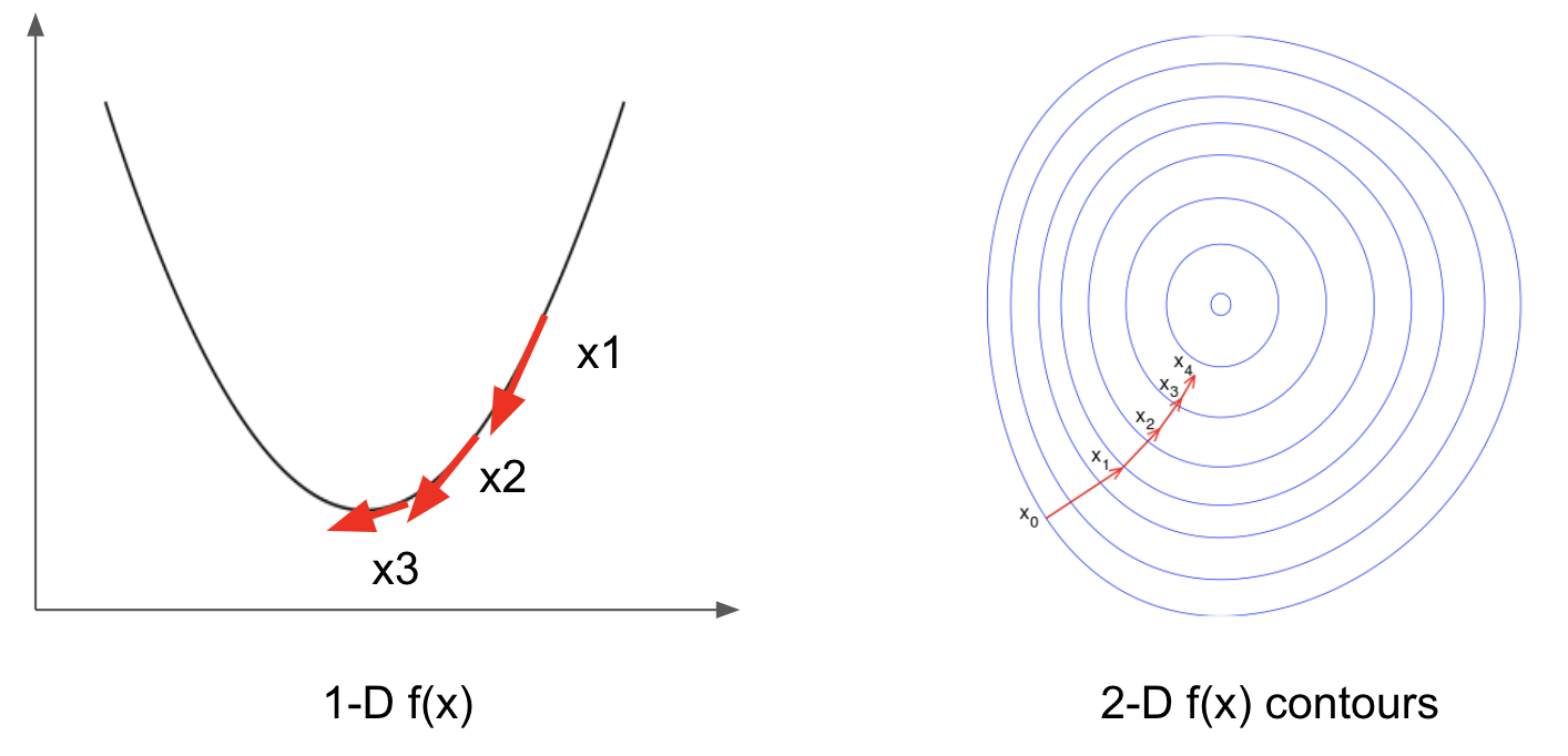
As shown in the figure, in 1-D case, \(p^k\) represents the tangential of function \(f\) and takes opposite direction from the gradient at \(x^k\). In 2-D case, function \(f\) is usually depicted by its contours and \(p^k\) is orthogonal to the contours [5].
The steepest descent algorithm uses
\(p^k = – \nabla f(x^k)^T \tag{11}\)
This means in equation 7, we have:
\(B = I \tag{12}\)
The optimal step length: search or not search
If you recall the implementation of logistic regression, we use a fixed value of step length of 1. Using too large a step length could lead to non-convergence, and too small a step length could lead to slow convergence. In theory, we can perform a 1-D search such that
\(\min_{\alpha >0} \phi (\alpha) \tag{13.1} \)
\(\phi (\alpha) = f(x^k + \alpha p^k) \tag{13.2}\)
Solving equation 13.1, we achieve the maximum benefit (decrease) of moving along \(p^k\).
We can use iterative golden-section search and interpolation to search the minimum [2]. In practice, however, a precise 1-D search can be expensive and slow, and most of the time we only need an approximate to achieve sufficient reduction of \(f\). There are several approaches to approximate step length [1], which I won’t cover here.
The implementation of iterative gradient descent methods usually does not perform search for the optimal step length at each step. Alternatively, we may treat step length as a hyperparameter to tune in model training and use a fixed value for each model, or we may adaptively modulate step length at each step.
Configuring learning rate is critical in training complex models such deep neural network, and latest development such as momentum, adaptive learning rate, learning rate schedule has been shown to improve the optimization process [3][4]. I will discuss more about learning rate later in deep learning posts.
Algorithm
Termination condition is defined by tolerance \(\epsilon >0\), see previous post.
- initiate \(x^0\)
- while termination condition not met:
- compute \(p^k = – \nabla f(x^k)\)
- compute \(\alpha^k = \min_{\alpha >0} f(x^k + \alpha p^k)\) or use a fixed value of \(\alpha\)
- \(x^{k+1} = x^k + \alpha^k p^k\)
- \(k = k+ 1\)
- return \(x^k, f(x^k)\)
When using precise search for step length \(\alpha^k\), from equation 13.1, we get
\(\nabla \phi (\alpha)= 0 \tag {14.1}\)
\(\nabla \phi (\alpha) = \nabla f(x^k + \alpha p^k)^T p^k = 0 \tag {14.2}\)
In the next iteration,
\(p^{k+1} = -\nabla f(x^{k+1}) = – \nabla f(x^k + \alpha p^k) \tag{15}\)
Therefore, from equation 14.2 and 15, we have
\((p^{k+1})^T p^k =0 \tag{16.1}\)
\(\nabla f(x^{k+1})^T \nabla f(x^{k}) =0 \tag{16.2}\)
This means using steepest descent, the search directions of consecutive steps are orthogonal, as shown in the figure below [1].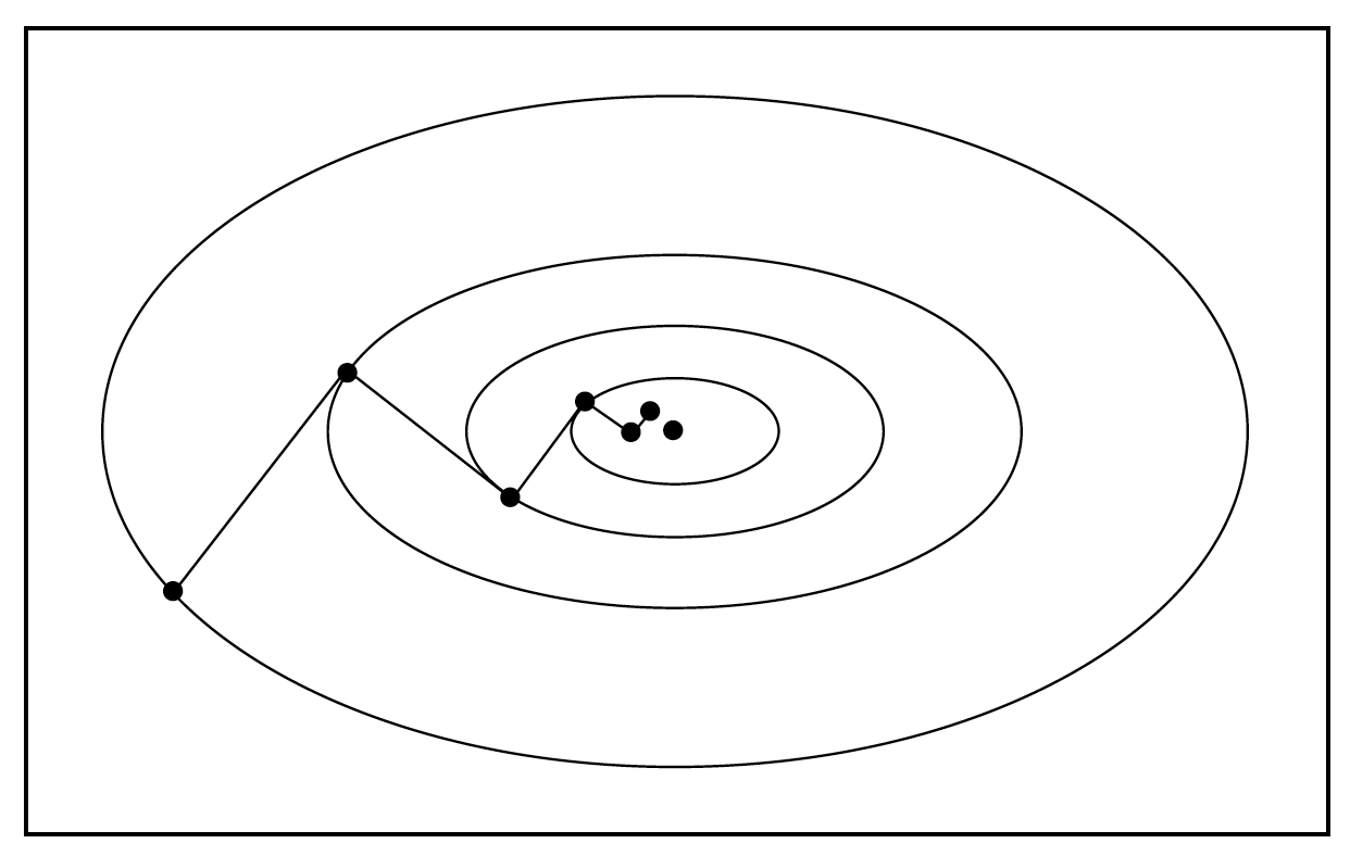
As a result of this zig-zag search manner, steepest descent achieves most rapid local descent, it may not achieve the most rapid global descent.
Newton method
If \(f(x)\) is continuously twice differentiable, using Taylor theorem, we have:
\(f(x^k + p^k) = f(x^k) + \nabla f(x^k)^T p^k + \frac{1}{2}(p^k)^T \nabla ^2 f(x^k)p^k + o\|p^k \|^2\tag{17} \)
\(p^k = \min_p m(p) \tag{18.1}\)
\(m(p^k) = f(x^k + p^k) \tag{18.2}\)
\(\nabla m(p^k) = \nabla f(x^k) + \nabla^2 f(x^k) p^k = 0 \tag{19}\)
\(\nabla ^2 f(x^k) \in R^{n \times n}\) is a symmetric square matrix of second derivatives of \(f\). If \(\nabla ^2 f(x^k)\) is non-singular, from equation 19, we can derive:
\(p^k = – (\nabla^2 f(x^k))^{-1}\nabla f(x^k) \tag{20} \)
We can write first and second derivatives as:
\(g = \nabla f(x), H = \nabla^2 f(x) \tag{21}\)
\(p^k\) is a descent direction, only if Hessian matrix \(H\) is positive definite and satisfies \(x^THx > 0\). Combining equation 20 and 21, we have
\(\nabla f(x^k)^T p^k \\= – \nabla f(x^k)^T (\nabla^2 f(x^k))^{-1} \nabla f(x^k)\\ = – g^T H^{-1} g < 0\tag{22}\)
This means in equation 7, we have:
\(B = \nabla^2 f(x^k) \tag{23}\)
Algorithm
- initiate \(x^0\)
- while termination condition not met:
- compute \(p^k = – (\nabla^2 f(x^k))^{-1}\nabla f(x^k) \)
- \(x^{k+1} = x^k + p^k \)
- \(k = k+1\)
- return \(x^k, f(x^k)\)
Note the step length is set as 1 for Newton Method. It is also possible to perform 1-D search for the optimal step length as done in steepest descent.
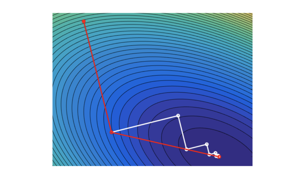
Shown in the figure at the beginning of this post are steepest descent (white lines) and Newton method (red lines) [6]. Compared with steepest descent, Newton method converges faster when the initial selection of \(x^0\) is close enough to the minimum \(x^{*}\). However, computation of Hessian matrix and its inverse can be expensive and slow. In addition, if \(x^0\) is too far away from \(x^{*}\), \(x^k\) may not converge.
In practice, steepest descent is more commonly used in function optimization given its advantage in computation.
Other not-so-common methods
Quasi-Newton
To avoid computation of Hessian matrix, we can replace the true Hessian with an approximation \(B^k\), which makes use of the first gradient to gain knowledge of the second derivative [1].
Conjugate gradient
The conjugate gradient method is used to solve linear optimization problems when the objective function has a quadratic format:
\(f(x) = \frac{1}{2}x^TAx + b^Tx \tag{24}\)
From equation 16.1 in steepest descent, we know that \(p^k, p^{k+1}\) are orthogonal. We may also construct a series of directions \(p^0, p^1, … p^{n-1}\) such that \(p_i, p_j\) are conjugate with respect to a positive definite symmetric matrix \(A\):
\(p_i^TAp_j = 0, i \neq j \tag{25.1}\)
\(p_i^TAp_i > 0 \tag{25.2}\)
\(p^0, p^1, … p^{n-1}\) are also linearly independent.
The first derivative of equation 24 is
\(\nabla f(x) = Ax + b \tag{26} \)
With limited steps \(n\), we can reach convergence.
\(\nabla f(x^n) = Ax^n + b = 0 \tag{27} \)
The construction of conjugate coordinates is flexible. Usually, we can initiate \(p^0\) based on gradient, and construct subsequent \(p^{k+1}\) using \(p^k\) and first derivatives at both \(x^k\) and \(x^{k+1}\), which I won’t cover here.
Algorithm
Termination condition: \(\nabla f(x^k) = 0\)
- initiate \(x^0, k = 0\)
- compute \(p^0 = – \nabla f(x^0)\)
- while termination condition not met:
- compute \(\alpha^k = \min_{\alpha >0} f(x^k + \alpha p^k)\) or use a fixed value of \(\alpha\)
- \(x^{k+1} = x^k + \alpha^k p^k\)
- \(p^{k+1} = – \nabla f(x^{k+1}) + \upsilon ^k p^k\), \(\upsilon^k = \frac{\|\nabla f(x^{k+1}) \|^2} {\|\nabla f(x^{k}) \|^2} \)
- \(k = k+1\)
- return \(x^{k+1}, f(x^{k+1})\)
What about gradient-free functions?
All of the methods discussed so far compute first derivative of function \(f\) (gradient). What if \(f\) does not have a explicit format and we do not know its gradient?
Gradient-free functions are essentially a black box and there are several commonly used methods for black-box optimization including grid search, genetic algorithm, simulated annealing, and Bayesian Optimization. I will discuss Bayesian Optimization in later post.
References
[1] Numerical Optimization, Jorge Nocedal, Stephen J. Wright
[2] https://github.com/wzhe06/Ad-papers/blob/master/Optimization%20Method/%E9%9D%9E%E7%BA%BF%E6%80%A7%E8%A7%84%E5%88%92.doc
[3] learning rate https://machinelearningmastery.com/learning-rate-for-deep-learning-neural-networks/
[4] momentum https://distill.pub/2017/momentum/
[5] wikipedia https://en.wikipedia.org/wiki/Gradient_descent
[6] wikipedia https://it.wikipedia.org/wiki/Metodo_del_gradiente_coniugato