
In machine learning, we are often dealing with high-dimension data. For convenience, we often use matrix to represent data. Numerical optimization in machine learning often involves matrix transformation and computation. To make matrix computation more efficiently, we always factorize a matrix into several special matrices such as triangular matrices and orthogonal matrices. In this post, I will review essential concepts of matrix used in machine learning.
This is No.7 post in the Connect the Dots series. See full table of contents.
While some matrix concepts may not seem intuitive, the goal of introducing matrix in numerical optimization and machine learning is of course NOT to confuse and intimidate non-mathematicians, but to represent high-dimension problems more conveniently and concisely. In addition, “smart” matrix transformation, factorization, decomposition can make matrix computation much more efficient.
Table of Contents
Two questions in linear algebra
There are essentially 2 questions in linear algebra and matrix:
- solve linear equation \(Ax = b\)
- eigendecomposition and singular value decomposition of a matrix \(A\)
In this post, I will discuss the first question, and in the next post, I will focus on the second one.
Matrix rank, inverse, singular, and determinant
Before we dive deep into matrix transformation, I would like to first review common matrix characteristics.
Rank
The rank of a matrix \(A\) is the maximal number of linearly independent columns in \(A\), which is equal to the row rank. See [1] for detailed description.
A matrix has full rank if its rank equals the large possible dimension:
$$ rank(A) = \min (m, n), A \in R^{m \times n} $$
For a square matrix \(A\), \(A\) is invertible if and only if \(A\) is full rank, i.e.
$$ rank(A) = n$$
Invertible
A square matrix \(A \in R^{n \times n} \) is invertible if there exists a matrix \(B \in R^{n \times n} \) such that
$$ AB = BA = I_n $$
The inverse of a matrix is written as \(A^{-1}\) .
Matrix \(A\) is not invertible if \(A\) is not full rank.
Singular
A square matrix \(A\) is also called singular if it is not invertible.
Determinant
The determinant of a square matrix \(A\) is a scalar value calculated from elements in \(A\). See [2] for detailed description.
\(A\) is singular and not invertible, if and only if its determinant \(det(A)\) is 0.
Solve linear equation \(Ax = b \)
1. Least square method in matrix format
\(A \in R^{m \times n}\) is a known matrix, \(x \in R^{n} \) is unknown, \(b \in R^{n \times 1}\) is a known vector. Linear regression uses a slightly different notation: \(A \in R^{n \times p}\) with \(n\) as the number of data points (rows), and \(p\) as the number of dimensions for each data point (columns).
Using the traditional notation, in linear regression optimization, the objective function sum of squared error can be written as:
\(J(x) = \min_{x \in R^n} \| Ax – b \|^2 \tag{1} \)
\(x^{*} = argmin_{x \in R^n} \| Ax – b \|^2 \tag{2}\)
With the linear regression notation, we have
\(\hat \beta = argmin_{\beta \in R^p} \| \textbf{X} \beta – y \|^2 \tag{3} \)
(1) \(m = n\)
When \(m = n\), \(A\) is a square matrix. If \(A\) is invertible, i.e. \(A\) is not singular, Equation 2 is equivalent to solving the linear equation \(Ax = b\), and we have a unique solution:
\(x^{*} = A^{-1}b \tag{4} \)
(2) \(m > n\)
Equation 4 looks quite different from what we derive in linear regression:
\(\hat \beta = ( \textbf{X}^T \textbf{X}) ^ {-1} \textbf{X}^Ty, \textbf{X} \in R^{n \times (p+1)} \tag {5} \)
The reason is that usually we have \(m > n\), i.e. there are more data points than feature dimension, the problem is called “overdetermined” and solution may not exist.
In this case, a solution to \(Ax = b\) is defined as the stationary point of the objective function \(J(x)\) from equation 1 and is computed by setting the first order derivative of \(J(x)\) as 0:
\(\frac {\partial J }{\partial x} = 2A^TAx – 2A^T b = 0 \tag {6.1}\)
\(A^TAx = A^Tb \tag {6.2}\)
If \(A^TA\) is invertible, we derive the same format of equation 5 as in linear regression:
\(x^{*} = (A^TA)^{-1}A^Tb \tag {7}\)
(3) \(m < n\)
When \(m < n\), there are more feature dimensions than data points, the problem is called “underdetermined” and the solution may be not unique. In this case, we define the solution x* as:
\(x^{*} = argmin_{Ax = b} \frac {1}{2}\|x\|^2 \tag {8} \)
Equation 8 is essentially an equality constrained optimization problem and we can solve it using Lagrange multiplier as discussed in later numerical optimization posts.
You may have seen similar expression of Equation 8 in regularization. Indeed, regularization is often used when \(n \gg m\) to reduce dimension.
(4) Geometric interpretation of least squares
Equation 1 can be interpreted as the finding the minimal Euclidean distance between 2 vectors: \(Ax\) and \(b\).
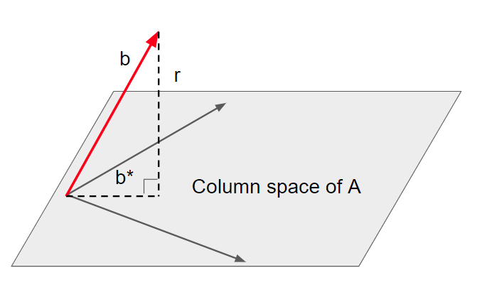
The minimal distance is achieved when we project \(b\) on the column space of \(A\):
\(b^{*} = Ax^{*} \tag{9}\)
We can write \(b\) as:
\(b = b^{*} + r, r \bot b^{*} \tag{10.1} \)
\(b = Ax^{*} + r, r \bot Ax^{*} \tag{10.2} \)
Therefore, \(x^{*} \) is a solution if and only if \(r\) is orthogonal to the column space of \(A\):
\(A^T r = 0, r = b – Ax \tag{11}\)
\(A^T(b-Ax) = 0 \tag{12.1} \)
$$A^TAx = A^Tb \tag {12.2}$$
Note that although equation 12.2 has the same format as equation 6.2, equation 12.2 is applicable to all least square problems for all possible \(m, n\). There is always a solution to equation 12.2, and the solution is unique if \(A\) is full rank [3].
Equation 12.2 can be written as \(A_1x = b_1\)
$$A_1 = A^TA, b_1 = A^Tb \tag {13}$$
\(A_1 \in R^{n \times n}\) is a square matrix.
Now, let’s rewrite equation 13 and substitute some letter notations in the general format of
$$Ax = b$$
2. Gaussian elimination in \(Ax = b\)
This is the most basic approach in solving a linear equation. The idea is to successively eliminate unknowns from equations, until eventually we have only one equation in one unknown. See reference [4][5] for well-elaborated examples.
If the square matrix \(A \in R^{n \times n}\) does not have full rank, then there is no unique solution.
Gaussian elimination includes 2 stages:
Stage 1: forward elimination
step \((k)\): eliminate \(x_k\) from equation \(k+1\) through n using multipliers:
\(m_{i,k} = \frac {a^{(k)}_{i,k}}{a^{(k)}_{k,k}}, i = k+1,k+2…n \tag{14} \)
Here we assume the pivot element \(a^{(k)}_{k,k} \neq 0\), although the original \(A\) may have 0 on its diagonal elements, we can permute \(Ax = b\) by swapping the order of equations for both \(A\) and \(b\) to make sure all pivot elements are not 0. The solution for a linear system is the same after permutation.
For example, we can permute:
$$\begin{bmatrix}
0 &1 \\
1& 2 \\
\end{bmatrix} \begin{bmatrix}
x_1 \\
x_2 \\
\end{bmatrix} = \begin{bmatrix}
3 \\
4 \\
\end{bmatrix} $$
to
$$\begin{bmatrix}
1 &2 \\
0& 1 \\
\end{bmatrix} \begin{bmatrix}
x_1 \\
x_2 \\
\end{bmatrix} = \begin{bmatrix}
4 \\
3 \\
\end{bmatrix} $$
and then we subtract the multiplier of row \(k\) from each row \(i\) in \(A\) and \(b\) and yield new matrix elements:
\(A^{(k)} x = b^{(k)} \tag{15} \)
At the end of stage 2, we have an upper triangular matrix \(A^{(n-1)}\), denoted as \(U\) and some new \(b^{(n-1)}\), denoted as \(g\):
\(Ux = g \tag{16} \)
The total cost: \(A \rightarrow U\) is approximately
$$\frac {2}{3}n^3$$
- division: \((n-1) + (n-2) … + 1 = \frac {n(n-1)}{2}\)
- multiplication: \((n-1)^2 + (n-2) ^2… + 1 = \frac {n(n-1)(2n-1)}{6}\)
- subtraction: \((n-1)^2 + (n-2) ^2… + 1= \frac {n(n-1)(2n-1)}{6}\)
Total cost: \(b \rightarrow g\) is approximately
$$ n^2 $$
- multiplication: \((n-1) + (n-2) … + 1 = \frac {n(n-1)}{2}\)
- subtraction: \((n-1) + (n-2)… + 1 = \frac {n(n-1)}{2}\)
Stage 2: back substitution
We solve equation 16 by back substitution from the last row to the first.
\(x_n = \frac {g_n}{u_{n,n}} \tag{17}\)
Total cost of solving \(Ux = g\) is approximately
$$ n^2$$
- division: n
- multiplication: \((n-1) + (n-2) … + 1 = \frac {n(n-1)}{2}\)
- subtraction: \((n-1) + (n-2) … + 1 = \frac {n(n-1)}{2}\)
The primacy cost of Gaussian elimination is thus to transform \(A\) to an upper triangular matrix \(U\).
3. LU factorization
Note that in linear algebra, we tend to use factorization and decomposition interchangeable, as they both mean breaking down a matrix into parts.
During Gaussian elimination, we can store the multipliers at each step to form a lower triangular matrix with diagonal values as 1 [4].
Thus, we can factorize a non-singular square matrix \(A\) into 2 triangular matrices with a permutation matrix:
$$ PA = LU \tag{18}$$
As discussed above, the cost of LU factorization is approximately
$$ \frac {2}{3}n^3$$
Another very desirable trait of triangular matrices is that their determinant is the product of the diagonal elements:
\(det(L) = 1, det(U) = \prod_i^n |u_{i,i}| \tag{19} \)
\(det(A) = det(L)det(U) \tag{20}\)
Thus we can compute determinant of \(A\) easily once we have its \(LU\) factorization.
To solve \(Ax = b\)
- factorize \(A = LU\), thus \(LUx = b\)
- solve \(d\) in \(Ld = b\), using forward substitution
- solve \(x\) in \(Ux = d\), using back substitution
4. Matrix inverse
\(AA^{-1} = I \in R^{n \times n} \tag{21}\)
\(I\) is an identity matrix with 1 on the diagonal and 0 everywhere else.
We may rewrite \(A^{-1}\) in column spaces. In the following example \(n = 2\):
\(A^{-1} = \begin{bmatrix}
a_1^{-1} & a_2^{-1}
\end{bmatrix} \tag{22.1}\)
\(a_1^{-1} =\begin {bmatrix}
x_{1,1}^{-1} \\ x_{1,2}^{-1}
\end{bmatrix}, a_2^{-1} = \begin{bmatrix} x_{2,1}^{-1} \\ x_{2,2}^{-1} \end{bmatrix} \tag{22.2}\)
We also rewrite \(I\) into \(n\) vectors:
\(I = \begin{bmatrix}
e_1 & e_2
\end{bmatrix} \tag{23.1}\)
\(e_1 =\begin {bmatrix}
1 \\ 0
\end{bmatrix}, e_2 = \begin{bmatrix} 0 \\ 1 \end{bmatrix} \tag{23.2}\)
We then just need to solve \(n\) linear systems separately to get each column \(a_i^{-1} \) in \(A^{-1}\):
\(Aa_i^{-1} = e_i, i = 1,2..n \tag{24}\)
5. Cholesky factorization
If \(A\) is a symmetric matrix:
\(A = A^T \tag{25}\)
We can improve the factorization and reduce the cost by half to \(\frac {1}{3}n^3\) because
\(A = LL^T \tag{26}\)
Note that \(L\) here, although is still a lower triangular matrix, does not have its diagonal elements as 1, as in equation 19. Thus \(L\) in Cholesky factorization is not the same as \(L\) in LU factorization.
To solve \(Ax = b\):
- factorize \(A = LL^T\), thus \(LL^Tx = b\)
- solve \(d\) in \(Ld = b\), using forward substitution
- solve \(x\) in \(L^Tx = d\), using back substitution
6. QR factorization
Both LU and Cholesky factorization only apply to square matrices. For rectangular matrices \(A \in R^{m \times n}\), we can use QR factorization:
\(A = QR \tag{27}\)
\(Q\) is a \(m \times m \) square orthogonal matrix, and its columns are orthogonal unit vectors:
\(QQ^T = Q^TQ = I, Q^T = Q^{-1} \tag{28}\)
\(R\) is a \(m \times n\) upper triangular matrix.
Again we can use permutation matrix \(P\) for column pivoting.
Similar to LU and Cholesky factorization, QR factorization can also be used to solve linear system.
If \(A\) is square:
\(det(A) = det(Q) det(R) = det(R) = \prod_i^n |r_{i,i}| \tag{29}\)
To solve \(Ax = b\):
- factorize \(A = QR\), thus \(QRx = b\)
- solve \(d\) in \(Qd = b\), \(Q^{-1} = Q^T\)
- solve \(x\) in \(Rx = d\), using back substitution
Take home message
To solve linear systems more efficiently, we always factorize a matrix into several special matrices such as triangular matrices and orthogonal matrices.
Reference
[1] https://en.wikipedia.org/wiki/Rank_(linear_algebra)
[2] https://en.wikipedia.org/wiki/Determinant
[3] http://math.ecnu.edu.cn/~jypan/Teaching/MatrixComp/slides_ch03_ls.pdf
[4] http://homepage.divms.uiowa.edu/~atkinson/m171.dir/sec_8-1.pdf
[5] youtube https://www.youtube.com/watch?v=piCVWXWjjsg