During logistic regression, in order to compute the optimal parameters in the model, we have to use an iterative numerical optimization approach (Newton method or Gradient descent method, instead of a simple analytical approach). Numerical optimization is a crucial mathematical concept in machine learning and function fitting, and it is deeply integrated in model training, regularization, support vector machine, neural network, and so on. In the next few posts, I will summarize key concepts and approaches in numerical optimization, and its application in machine learning.
This is No.6 post in the Connect the Dots series. See full table of contents.
Table of Contents
1. The basic formula
$$ \min f(x) \tag {1.1} $$
$$ s.t. $$
$$ h_i(x) = 0, i \in 1,2…m \tag {1.2} $$
$$ g_j(x) \leq 0, j \in 1,2…n \tag{1.3} $$
\(f(x): R^n \rightarrow R\) is the objective function we want to optimize, and usually takes the format of “minimize”. For example, in linear regression, it has the format of \(f(\hat y_i) = \sum_i^N(y_i – \hat y_i)^2 \). If the goal is to maximize a function, just take the negative value of \(f\).
2. constrained v.s. constrained
Equation 1.1 is the basic format of an unconstrained numerical optimization problem.
Equation 1.2 and 1.3 represent conditions in constrained optimization problems. \(s.t.\) means subject to, and it is followed by the constraint functions. \(i, j\) are indices of constraint functions as an optimization problem may have several constraint functions. In particular, equation 1.2 is equality constraint and 1.3 is inequality constraint.
A set of points satisfying all constraints define the feasible region:
$$ K = \{x \in R^n | h_i(x) = 0, g_j(x) \leq 0 \} \tag{2} $$
The optimal point that minimizes the objective function is denoted as \(x^{*}\):
$$ x^{*} = argmin_{x \in R^n} f(x) \tag {3} $$
3. global v.s. local
\(x^{*}\) is the global minimum if
$$ f(x^{*}) \leq f(x), x \in K \tag {4.1} $$
\(x^{*}\) is a local minimum if within a neighborhood of \(\epsilon\):
$$ f(x^{*}) \leq f(x), \exists \epsilon>0, \|x^{*} – x\| \leq \epsilon \tag {4.2} $$
If \(f(x)\) is convex, a local minimum is also the global minimum.
4. continuous v.s. discrete
Some optimization problems require \(x\) to be integers. Therefore, rather than taking infinite real value, \(x\) can only take a finite set of values. It is usually more difficult to solve discrete optimization problems than continuous problems. See “linearity” below.
5. convexity
Convexity is a key concept in optimization. It guarantees a local minimum is also the global minimum.
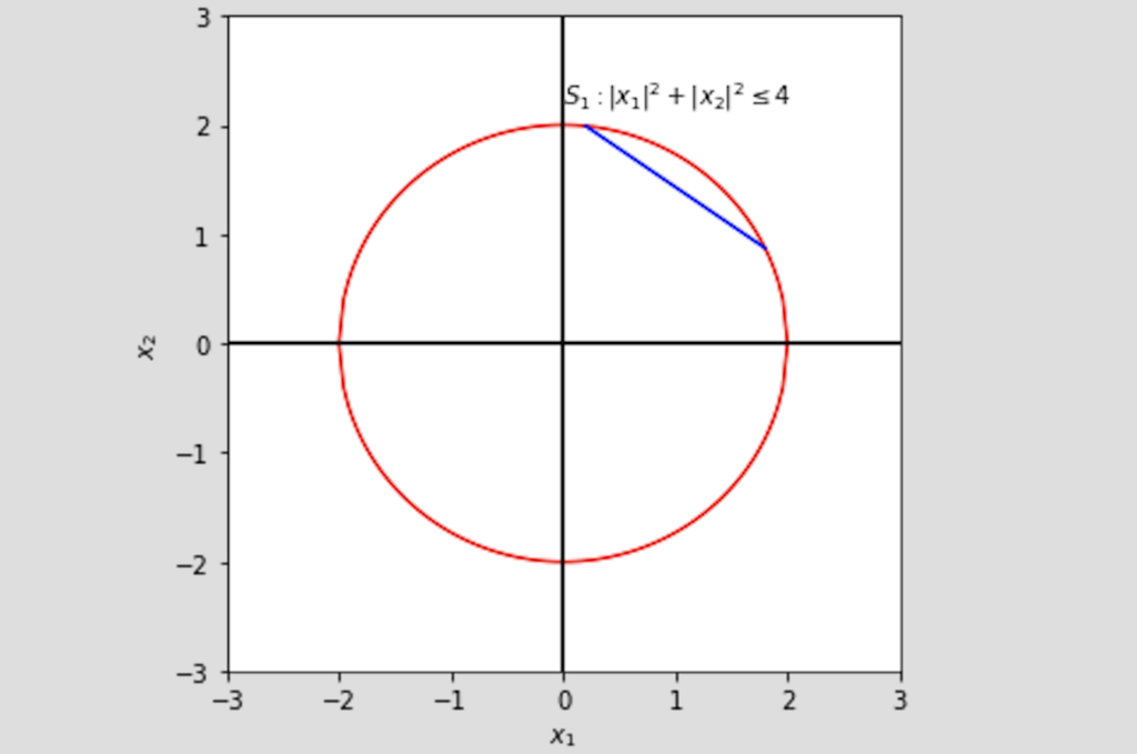
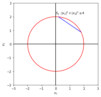
\(S\) is a convex set, if for any two points in \(S\):
\(\lambda x_1 + (1 – \lambda) x_2 \in S, \forall x_1, x_2 \in S, \lambda \in [0,1] \tag {5} \)
In the figure below, areas enclosed by the red curves represent set \(S\). \(S_1\) is convex and \(S_2\) is not convex, as a straight line (blue) connecting \(x_1, x_2\) is not within \(S_2\).

\(f\) is a convex function if its domain \(S\) is a convex set and if for any two points in its domain:
\(f(\lambda x_1 + (1 – \lambda) x_2) < \lambda f( x_1) +(1 – \lambda) f(x_2),\forall x_1, x_2 \in S, \lambda \in [0,1] \tag {6} \)
As discussed in the logistic regression post, a twice continuously differentiable function \(f\) is convex if and only if its second order derivative \(f”(x) \geq 0\). In matrix format, it means its Hessian matrix of second partial derivatives is positive semidefinite. That is why we need to use maximum likelihood, rather than squared error as the error function in logistics regression.
\(f\) is concave if \(-f\) is convex.
6. linearity
If \(f(x), h(x), g(x)\) are all linear function of \(x\), the problem is a linear optimization problem (also called linear programming). If any function is non-linear, the problem is a non-linear optimization problem.
Continuous and integer linear optimization problems have different complexity. Continuous linear optimization problems are in P, which means it can be solved in polynomial time. Integer linear optimization is NP-complete (Nondeterministic polynomial), which means we can verify whether a given solution is correct or not in polynomial time, but it is uncertain whether we can solve the problem ourselves in polynomial time [3]. I will discuss P v.s. NP in detail in later posts.
7. iterative algorithm
As in logistic regression, numerical optimization algorithms are iterative, with a sequence of improved estimates \(x_k, k = 1,2,…\) until reaching a solution. In addition, we would like to go towards a descent direction such that:
\(f(x_{k+1}) < f(x_k) \tag{7}\)
The termination condition is defined by a small threshold \(\epsilon\) with any the following format:
1. the change of input is small
$$ \|x_{k+1} – x_{k} \| < \epsilon \tag{8.1} $$
$$ \frac { \|x_{k+1} – x_{k} \|}{ \|x_k \|} < \epsilon \tag{8.2} $$
2. the decrease of the objective function is small
$$f(x_{k+1}) – f(x_k) < \epsilon \tag{9.1}$$
$$ \frac{f(x_{k+1}) – f(x_k)}{|f(x_k)|} < \epsilon \tag{9.2}$$
Note that because \(x \in R^n\) is a vector, the distance between 2 vectors is defined by the norm, such as Euclidean distance, and the magnitude of a vector is defined by its norm. \(f\) is a scalar, and thus its magnitude is defined by its absolute value.
A good algorithm should have the following properties [1]:
- robust: work well with reasonably choices of initial values for various problems
- efficient: not require too much computing time, resource, and storage
- accurate: identify a solution with high precision, and not over sensitive to noise and errors
Usually, an efficient and fast converging method may require too much computing resource, while a robust method could be very slow. A highly accurate method may converge very slow and less robust. In practice, we have to consider the trade-off between speed and cost, between accuracy and storage [1].
8. Taylor’s theorem
I first learned about Taylor’s theorem back in college and have been taking its application for granted. While the basic format of Taylor’s theorem is simple, it plays a central role in numerical optimization. Thus, I would like to recap some key ideas in Taylor’s theorem.
The idea of Taylor’s theorem is to approximate a complex non-polynomial by higher order polynomials, using a series of simple k-th order polynomials, called Taylor polynomials. Taylor polynomials are finite-order truncation of Taylor series, which completely defines the original function in a neighborhood.
The simplest case is first-order 1-dimension Taylor’s theorem [4], which is equivalent to Lagrange’s Mean Value Theorem [5]:
If \(f\) is continuous on interval \([a,x]\) and \(f\) is differentiable on \((a,x)\), then there exists a point \(b: a<b<x\) such that
$$f'(b) = \frac {f(x) – f(a)}{x-a} \tag {10.1}$$
$$f(x) = f(a) + f'(b)(x-a) \tag {10.2}$$

If \(a\) is close enough to \(x\), thus \(f'(b) \approx f'(a)\), equation 10.2 can be written as:
$$f(x) \approx f(a) + f'(a)(x-a) \tag {11}$$
Thus, \(f(x)\) can be approximated by a linear function.
Similarly, if \(f(x)\) is twice differentiable, we can approximate it as:
$$f(x) \approx f(a) + f'(a)(x-a) + \frac {1}{2}f”(a)(x-a)^2\tag {12}$$
If \(f(x)\) is infinitely differentiable, such as \(e^x\), its Taylor series in a neighborhood of value \(a\) can be written as the following:
$$f(x) = \sum_{n=0}^{\infty} \frac {f^{(n)}(a)}{n!} (x-a)^n \tag{13}$$
\(n!\) is the factorial of n, and \(f^{(n)}(a)\) denotes the \(n\)th derivative of \(f\) at point \(a\). When \(a= 0\), it is called Maclaurin series:
$$f(x) = \sum_{n=0}^{\infty} \frac {f^{(n)}(0)}{n!} (x)^n \tag{14}$$
For example, expanding \(e^x\) at 0 we can get
$$e^x = \sum_{n=0}^{\infty} \frac {1}{n!} x^n \tag{15} $$
When we only consider the first k-th order of derivatives, we have an approximation of \(f(x)\) as
$$f(x) \approx \sum_{n=0}^{k} \frac {f^{(n)}(a)}{n!} (x-a)^n \tag{16}$$
In practice, we usually expand a function to its 1st or 2nd order derivative to get a good enough approximation of a function.
In matrix format, equation 11 can be written as
\(f(x) \approx f(a) + (x-a)^T \nabla f(a) \tag{17}\)
Equation 12 can be written as
\(f(x) \approx f(a) + (x-a)^T \nabla f(a) + \frac{1}{2}(x-a)^TH(a)(x-a) \tag{18} \)
Here, \(\nabla\) denotes first order derivative Jacobian matrix, and \(H\) denotes second order partial derivative Hessian matrix.
In the case of numerical optimization, as we will see in the next post, Taylor first order polynomial will give us a good clue about the direction to move \(x_k\) to \(x_{k+1}\). And Taylor second order polynomial will give us useful information about convexity.
References
[1] Numerical Optimization, Jorge Nocedal, Stephen J. Wright
[2] https://github.com/wzhe06/Ad-papers/blob/master/Optimization%20Method/%E9%9D%9E%E7%BA%BF%E6%80%A7%E8%A7%84%E5%88%92.doc
[3] https://cs.stackexchange.com/questions/40366/why-is-linear-programming-in-p-but-integer-programming-np-hard
[4] https://www.rose-hulman.edu/~bryan/lottamath/mtaylor.pdf
[5] https://en.wikipedia.org/wiki/Mean_value_theorem