Why do we care about eigenvalues, eigenvectors, and singular values? Intuitively, what do they tell us about a matrix? When I first studied eigenvalues in college, I regarded it as yet another theoretical math trick that is hardly applicable to my life. Once I passed the final exam, I shelved all my eigen-knowledge to a corner in my memory. Years have passed, and I gradually realize the importance and brilliance of eigenvalues, particularly in the realm of machine learning. In this post, I will discuss how and why we perform eigendecomposition and singular value decomposition in machine learning.
This is No.8 post in the Connect the Dots series. See full table of contents.
In the previous post, I mentioned that there are essentially 2 questions in linear algebra and matrix:
- solve linear equation \(Ax = b\)
- eigendecomposition and singular value decomposition of a matrix \(A\)
Here I will focus on the second one.
Table of Contents
Eigendecomposition and singular value decomposition
Matrix is all about transformation and change of coordinate systems. Through rotation, stretch, and scale, we can reveal unique characteristics of a matrix, and decompose a matrix into simple and representative matrices.
1. Eigendecomposition
Also called Eigen Value Decomposition (EVD) [1].
Geometric interpretation of EVD
This video by 3Blue1Brown provides a very informative geometric interpretation of EVD.
Essentially, when we linearly transform a matrix by stretch and rotate, if a vector \(v \in R^{n}\) in the space changes only by a scalar factor \(\lambda\) after transformation, we call such vector an eigenvector.
\(Av = \lambda v \tag{1} \)
Eigenvalues are be used directly to calculate the determinant of a matrix:
\(det(A) = \prod_i^n |\lambda_i|\tag{2}\)
\(A\) is singular if its eigenvalues is 0.
Eigendecomposition
If a square matrix \(A \in R^{n \times n}\) has \(n\) linearly independent eigenvectors \(q_i \in R^{n}\).
For a single eigenvector \(q_i\), from equation 1, we have
\(Aq_i = \lambda_i q_i, i = 1,2…n \tag{3} \)
For all eigenvectors, we can define a square matrix \(Q \in R^{n \times n}\) with \(q_i\) in each column:
\(Q = \begin{bmatrix} q_1 & q_2 & … &q_n \end{bmatrix} \tag{4} \)
For all eigenvalues, we can define a diagonal matrix \(\Lambda \in R^{n \times n}\) with the eigenvalues \(\lambda_i\) as the diagonal elements:
\(\Lambda = diag(\lambda_1, \lambda_2, … \lambda_n) \tag{5} \)
Thus equation 3 with all eigenvalues and eigenvectors of \(A\) can be written as:
\(AQ = Q \Lambda \tag{7}\)
Because all eigenvectors are linearly independent, \(Q\) has full rank and invertible with inverse \(Q^{-1}\)
\(AQQ^{-1} = Q \Lambda Q^{-1} \tag{8}\)
Therefore, we can decompose a full rank square matrix \(A\) into square matrices of eigenvectors and a diagonal matrix with eigenvalues [5].
\(A = Q \Lambda Q^{-1} \tag{9} \)
If \(A \in R^{n \times n}\) does not have \(n\) linearly independent eigenvectors, then it is not diagonalizable. In this case, \(A\) is also called defective matrix, and there is no diagonal matrix \(\Lambda\) for eigendecomposition in equation 9.
2. Singular value decomposition SVD
LU factorization and eigendecomposition mentioned before are only applicable to square matrices. We would like to have a more generic decomposition approach for any rectangular matrices.
Geometric interpretation of SVD
We start with a \(R^n\) space defined by orthogonal unit vectors \(v\). Shown in the figure above is a 2-dimension example. Note that \(v_1, v_2\) are unit vectors \(\|v_i\| = 1\), and they define a sphere \(S\) [2][3].
Now we apply a linear transformation \(A \in R^{n \times n} \) to transform the sphere \(S\) into an output space \(AS \in R^{n \times n}\) . In this new space, the original sphere \(S\) is transformed into an ellipse defined by 2 unit vectors \(u_1, u_2\), with scalar factors of \(\sigma_1, \sigma_2\) respectively.
Therefore, we have
\(Av_i = \sigma_i u_i \tag {10}\)
Note that equation 10 looks quite similar to eigendecomposition in equation 3, except that \(v_i \neq u_i\).
We can rewrite equation 10 in a matrix format with all \(n\) dimension of \(A\):
\(AV = \hat U \hat {\Sigma} \tag{11} \)
\(V = \begin{bmatrix} v_1 &v_2 & … &v_n \end{bmatrix} \tag{12} \)
\(\hat U = \begin{bmatrix} u_1 & u_2 & … &u_n \end{bmatrix} \tag{13} \)
\(\hat {\Sigma} = diag (\sigma_1, \sigma_2, … \sigma_n) \tag{14}\)
\(\hat {\Sigma}\) is a diagonal matrix with sorted diagonal values of \(\sigma_i\), called singular values:
\(\sigma_1 \geq \sigma_2 .. \geq \sigma_{\min(m,n)} \geq 0 \tag{15} \)
Geometrically, \(V\) is an orthonormal matrix defining in the input space:
\(VV^T = V^TV = I, V^T = V^{-1}, det(V) = 1 \tag{16.1}\)
In theory, \(V\) can take either real or complex values. In the case of complex values, \(V\) is called an unitary matrix with its conjugate transpose \(V^{*}\):
\(VV^{*} = V^{*}V = I\tag{16.2}\)
\(A\) is a linear transformation matrix.
\(\hat U\) represents orthogonal vectors as the rotation of the input space, and \(\hat {\Sigma}\) represents stretch.
We can rewrite equation 11 in the real value case as:
\(AVV^T = \hat U \hat {\Sigma}V^T \tag{17} \)
\(A = \hat U \hat {\Sigma}V^T \tag{18.1} \)
In the complex value case, we can write it in the following format:
\(A = \hat U \hat {\Sigma}V^{*}\tag{18.2} \)
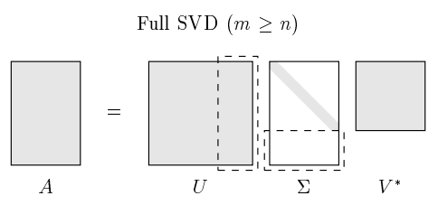
Equation 18 is called reduced singular value decomposition, with \(\hat {\Sigma}\) as a square diagonal matrix. Usually, we can pad \(\hat {\Sigma}\) with zeros and add arbitrary orthogonal columns to \(\hat U\) to form an unitary matrix \(U\), \(UU^T = I\), as shown in the following figure:
\(A = U {\Sigma}V^T \tag{19.1}\)
\(A = U {\Sigma}V^{*} \tag{19.2}\)
Equation 19 is the general format of singular value decomposition. Any matrix \(A \in R^{m \times n}\) can be decomposed into these 3 matrices: \(U \in R^{m \times m}, V \in R^{n \times n}\) are orthogonal square matrices (also called unitary matrix if \(U,V\) takes complex values), \(\Sigma \in R^{m \times n}\) is a diagonal matrix.
SVD is commonly used in recommendation system and matrix factorization.
3. Covariance matrix, EVD, SVD
Covariance matrix \(C = A^TA\) is used to describe the redundancy and noise in data \(A\). For a matrix \(A \in R^{m \times n}\), multiplying it to its transpose gives us a square and symmetric matrix.
The diagonal elements represent variance of \(C\) and off-diagonal elements represent covariance. \(C\) is likely to be a dense matrix unless all columns in the input \(X\) are independent, i.e. covariance equals to 0.
Dense matrices are difficult to transform, inverse, and compute. If we can diagonalize a matrix such that all off-diagonal elements are 0, matrix computation would be easier and more efficient.
As discussed above, both EVD and SVD can diagonalize square matrices.
Using SVD, we have:
\(A^TA \\ = (U \Sigma V^T )^TU \Sigma V^T \\ =V {\Sigma}^T U^T U \Sigma V^T \\ = V{\Sigma}^T \Sigma V^T \\ = V {\Sigma}^2 V^T \tag {20} \)
Since \(V\) is unitary matrix, \(V^T = V^{-1}\), equation 20 can be written as:
\(A^TA = V {\Sigma}^2 V^{-1} \tag{21}\)
Similarly
\(AA^T = U {\Sigma}^2 U^T = U {\Sigma}^2 U^{-1} \tag{22} \)
Equation 21 and 22 have the same format as equation 9: eigendecomposition.
Indeed, if \(C\) is a symmetric matrix, its eigendecomposition is the same as its singular value decomposition. The eigenvectors of \(C\) are not only linearly independent, but also orthogonal.
Let the eigenvalues for \(C = A^TA\) be \(\Lambda\), we have:
\(\Lambda = {\Sigma}^2 \tag{23.1}\)
\(\lambda_i = {\sigma_i}^2 \tag{23.2} \)
Covariance matrix with singular value decomposition is used in Principal Component Analysis (PCA) [4], discussed in later posts.
4.Positive definite matrix
Another common matrix concept is positive definite. It is a characteristic of a symmetric matrix \(M \in R^{n \times n}\), such as covariance matrix \(A^TA\) and second derivative Hessian matrix \(\frac {\partial^2 J(x)}{\partial x}\). In optimization, the objective function is convex if Hessian matrix is positive definite.
One way to evaluate the definiteness of a matrix is to check its eigenvalues:
- if all eigenvalues are positive, \(M\) is positive definite.
- if all eigenvalues are negative, \(M\) is negative definite
- if all eigenvalues are non-negative, \(M\) is positive semi-definite
- if all eigenvalues are non-positive, \(M\) is negative semi-definite.
- else, \(M\) is indefinite.
Definiteness of a matrix is also evaluated in the following format.
- if \(x^TMx > 0,\forall x \in R^n\), \(M\) is positive definite.
\(M = Q \Lambda Q^{-1} \tag{24} \)
\(x^TMx = x^TQ \Lambda Q^T x = y^T \Lambda y \tag{25.1}\)
\(y= Q^T x \tag{25.2}\)
In equation 24, because \(\Lambda = diag(\lambda_1, \lambda_2, … \lambda_n) \):
\(x^TMx \\= y^T \Lambda y \\ = \sum_i^n (y_i)^2 \lambda_i \tag{26}\)
For a positive definite matrix \(M\), all eigenvalues are bigger than 0, \(\lambda_i > 0\), as a result:
\(x^TMx = \sum_i^n (y_i)^2 \lambda_i > 0 \tag{27}\)
Similarly,
- if \(x^TMx < 0, \forall x \in R^n\), \(M\) is negative definite.
- if \(x^TMx \geq 0 ,\forall x \in R^n\), \(M\) is positive semi-definite.
- if \(x^TMx \leq 0, \forall x \in R^n\), \(M\) is negative semi-definite.
- if \(x^TMx > 0, \exists x \in R^n. x^TMx < 0, \exists x \in R^n\), \(M\) is indefinite.
Take home message
Eigendecomposition and singular value decompositon factorize a matrix into a diagonal matrix, which not only reveals unique characteristics of the data, but also makes matrix computation more efficiently.
References
[1] https://en.wikipedia.org/wiki/Eigenvalues_and_eigenvectors
[2] http://www.cs.cornell.edu/courses/cs322/2008sp/stuff/TrefethenBau_Lec4_SVD.pdf
[3] youtube https://www.youtube.com/watch?v=EokL7E6o1AE
[4] https://intoli.com/blog/pca-and-svd/
[5] https://en.wikipedia.org/wiki/Orthogonal_matrix


