In my previous post, I presented interesting trips patterns of NYC taxis. Here, I focus my analysis of Brooklyn. Brooklyn is a very popular place of interest for both tourists and local people to eat, drink, and have fun. I usually take subway train L or G to visit Brooklyn. However, L train is to be shut down in 2019 for 1.5 years [1], which may severely affect Brooklyn’s business. Taxi trips, in particular, shared taxi trips, may become the mainstream transportation in Brooklyn.
To understand possible shared trip, I grouped pickup and dropoff locations by zipcode, neighborhood, and county. In order to do this, I first converted coordinates to address using Geocoder API for green taxi. Since the API is slow, I used single days (Wednesday, Saturday, Sunday) to represent weekday and weekends. I also included Uber data in this analysis, which include the pickup neighborhood information. Check my first post of data wrangling here.
Table of Contents
Trip within Brooklyn
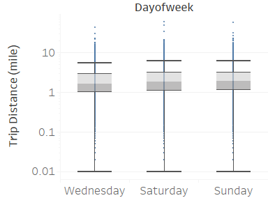
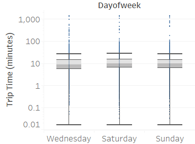
I first looked at trips starting and ending within Brooklyn. Such trips are defined as local trip and they usually have short distances of 2 miles and travel time 10 minutes.
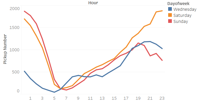
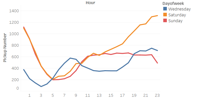
Weekday (Wednesday) pickup in Brooklyn peaked at 9 pm. Saturday pickup peaked at midnight, starting to increase in late afternoon, and lasted to Sunday morning. Sunday however, had a lower pickup late night (lower than Wednesday).
Where did taxi pick up and drop off passengers?


Animated pickup map by hour
Saturday Pickup in Brooklyn
The spatial temporal pattern revealed that evening and late weekend night were the busiest time for certain Brooklyn areas.
Top 10 zip codes for pickups are 11231, 11205, 11216, 11222, 11238, 11215, 11249, 11217, 11211, 11201
Top 10 zip codes for drop off are 11201, 11211, 11217, 11249, 11215, 11238, 11222, 11216, 11205, 11231
Top Neighborhoods
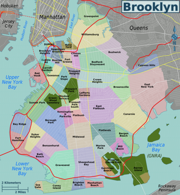
(image url https://en.wikipedia.org/wiki/File:Brooklyn_neighborhoods_map.png)
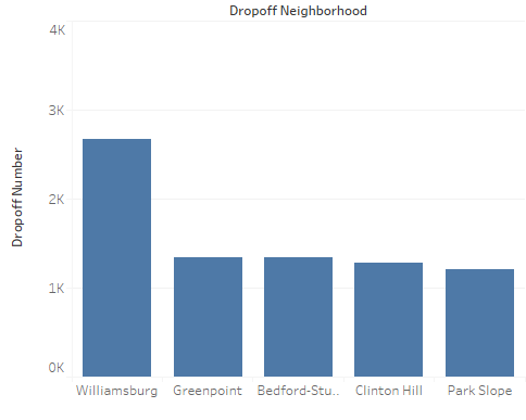
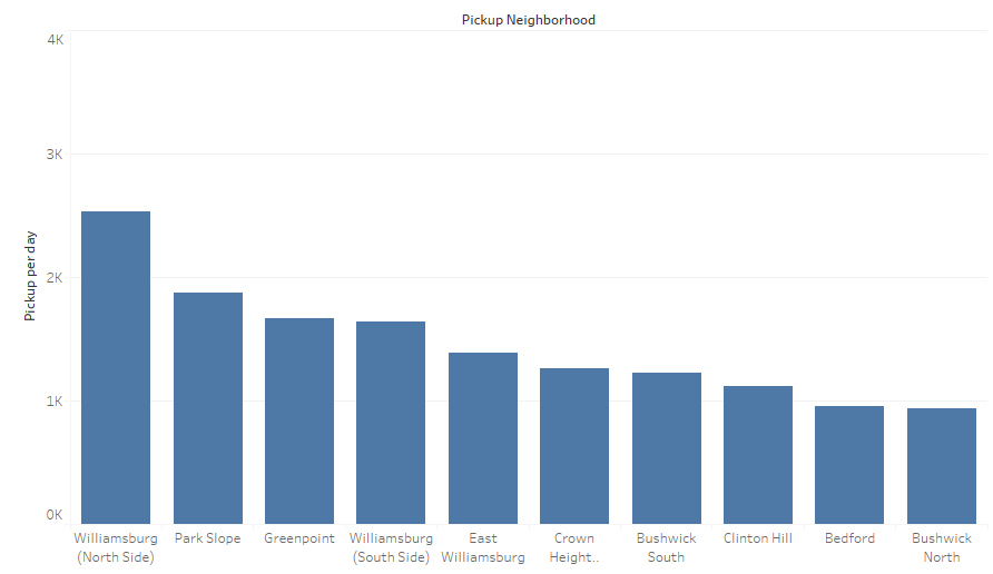
When I grouped trips by neighborhood names, the popular spots became familiar. Williamsburg, Greenpoint, Park Slope, Clinton Hill were hot pickup and drop off spots. In particular, Williamsburg led the 2nd popular spot by 100%.

Uber is also popular in these neighborhoods
I looked at Uber’s pick up records on the same days.
Similar to Green Taxi, Uber trip in Brooklyn also had a morning peak and a evening peak on Weekday. Yet trips droped in the middle of the day. On Saturday (Friday) overnight and Sunday overnight, there were more trips, similar as Green taxi.
Top neighborhoods of Uber, again, include Williamsburg, Park Slope, Greenpoint.
Popular Routes
Now that we know most trips start and end at similar hot spots, I then investigated popular routes in Brooklyn. If some routes are very popular, it may be possible to redesign bus/shuttle routes. Also, if passengers share the same routes, they may also share taxi rides, which only only help passengers to save money, but also increase the efficiency of taxi rides.
I started with Green taxi Saturday data and grouped trips by pickup and dropoff zip codes.
sat_route_zipcode = sat_bk_bk.groupby(['pickup_zipcode','dropoff_zipcode'],as_index=False).count()[['pickup_zipcode','dropoff_zipcode','pickup_datetime']]
sat_bk_bk_distance = sat_bk_bk.groupby(['pickup_zipcode','dropoff_zipcode'],as_index=False).mean()[['pickup_zipcode','dropoff_zipcode','trip_distance']]
sat_routes = sat_route_zipcode.merge(sat_bk_bk_distance)
sat_routes.sort_values('pickup_datetime',ascending=False,inplace=True)
sat_routes.rename(columns = {'pickup_datetime':'trip number'}, inplace=True)
sat_routes
	pickup_zipcode	dropoff_zipcode	trip number	trip_distance
1	11201	11201	542	0.989410
254	11211	11211	523	0.934589
265	11211	11222	517	1.243926
937	11249	11211	415	1.054024
540	11222	11211	353	1.300425
249	11211	11206	326	1.619724
948	11249	11222	326	1.163926
29	11201	11231	322	1.530280
16	11201	11217	320	1.289594
352	11215	11215	316	1.091582
279	11211	11249	286	1.002483
423	11217	11215	248	1.354758
962	11249	11249	234	0.743547
410	11217	11201	223	1.339327
4	11201	11205	221	1.522489
14	11201	11215	212	2.279104
354	11215	11217	197	1.170964
549	11222	11222	196	0.937908
264	11211	11221	194	2.662938
36	11201	11238	192	2.123646
563	11222	11249	187	1.270321
445	11217	11238	178	1.214775
932	11249	11206	176	2.181420
719	11231	11231	166	1.214699
10	11201	11211	165	3.591879
694	11231	11201	160	1.537688
246	11211	11201	156	3.810256
107	11206	11211	153	1.360523
425	11217	11217	144	0.840000
64	11205	11201	142	1.552254
...	...	...	...	...
486	11220	11214	1	3.120000
485	11220	11211	1	9.320000
482	11220	11205	1	8.690000
480	11220	11201	1	4.920000
478	11219	11230	1	3.300000
476	11219	11218	1	4.300000
554	11222	11228	1	11.690000
566	11223	11214	1	1.100000
625	11225	11234	1	4.030000
567	11223	11219	1	1.930000
618	11225	11224	1	2.050000
615	11225	11220	1	4.470000
606	11225	11209	1	7.450000
599	11224	11239	1	9.500000
597	11224	11236	1	8.080000
592	11224	11230	1	4.020000
585	11224	11221	1	3.430000
584	11224	11220	1	5.740000
582	11224	11212	1	10.200000
581	11224	11211	1	15.680000
580	11224	11210	1	6.100000
578	11224	11207	1	10.640000
577	11224	11205	1	15.100000
576	11224	11204	1	4.090000
575	11224	11201	1	12.580000
573	11223	11232	1	8.400000
572	11223	11230	1	2.050000
570	11223	11228	1	3.870000
569	11223	11226	1	4.350000
976	11417	11212	1	1.600000
From the list of popular routes above, I noticed that these trips had same or similar pick up and drop off zip codes, and short trip distance < 2 miles.
I defined shareable trips as trips with pickup time within 5 minutes and with same pickup and dropoff zipcodes. If there are more than 1 trip, number of shareable trips = total passenger number / 6, while 6 is the capability of each taxi. Otherwise, the number of non-shareable trip is 1, for each route and time window. Then for each pickup zipcode, I count the total number of shareable trips and non-shareable trips. Shared ride efficiency for each zipcode = #shareable trips / (#shareable+#non-shareable trips). Hourly ride efficiency is calculated as the mean efficiency across all zip codes.
1 Group by pickup and dropoff zipcode (namely route), and count total trip number, total passenger number, aggr trip number, and non aggr trip number. If total trip number of a certain route is 1, aggr is 0. Otherwise, divided the total number of passengers by 6 given that 6 is the capacity of a taxi. Non aggr trip is 0 when there is aggr trip, otherwise, it is 1.
def aggr_trip(df):
    df_gp = df.groupby(['pickup_zipcode','dropoff_zipcode'],as_index=False)
    df_trip_num = df_gp.count()[['pickup_zipcode','dropoff_zipcode','pickup_datetime']]
    df_passenger_num = df_gp.sum()[['pickup_zipcode','dropoff_zipcode','passenger_count']]
    df_eff = df_trip_num.merge(df_passenger_num)
    df_eff.rename(columns = {'pickup_datetime':'trip number'}, inplace=True)
    df_eff['aggr trip number'] = np.where(df_eff['trip number'] == 1,0,np.ceil(1.*df_eff['passenger_count']/6))
    df_eff['non aggr trip number'] = np.where(df_eff['trip number'] == 1,1,0)
    return df_eff
2.Calculate shared ride percentage across all areas
def aggr_eff(df):
    df_eff = aggr_trip(df)
    df2 = df_eff.groupby('pickup_zipcode',as_index=False).sum()[['pickup_zipcode','passenger_count','aggr trip number','non aggr trip number']]
    df2['aggr eff'] = 1.*df2['aggr trip number'] / (df2['aggr trip number'] + df2['non aggr trip number'] )
    return df2
3 Average across all routes
def aggr_eff_all(df):
    if df.empty:
        return 0
    else:
        df2 = aggr_eff(df)
        return df2['aggr eff'].mean()
4. ..
Overall, I defined hourly shared ride efficiency.

From my calculation, I reported that over 15% of trips on Saturday after 4 pm to Sunday 4 am are shareable. Over 10% of trips on Wednesday morning during rush hour are shareable.
Using similar analysis used above, I also analyzed trips between Brooklyn and Manhattan.
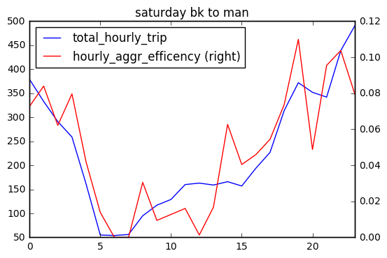
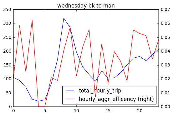
Total Hourly Trip and Shared ride efficiency
From my definition and calculation of hourly shared ride efficiency, it seems that shared ride efficiency should be correlated to total number of trips. The more trips there are, the more likely shared routes exist.
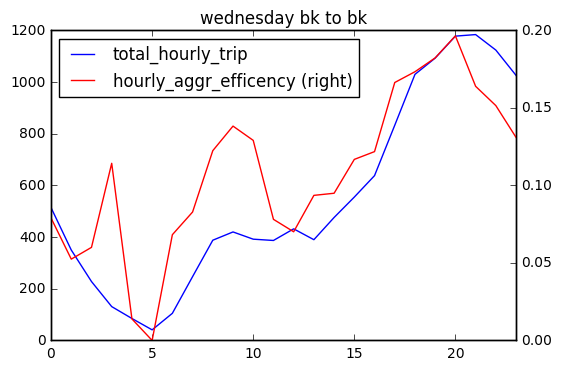
I plotted hourly shared ride efficiency and total hourly trip number of each day, and find that in general, share ride efficiency changes as total hourly trip number changes. There are several peaks in hourly share ride efficiency (red). Sat 1 am, 2 am, 8 pm; Sun 1-2 am (prolonged peak at midnight) ; Wednesday 3 am and 9 am. These peaks may suggest that at certain time, passengers are more likely go to similar direction.

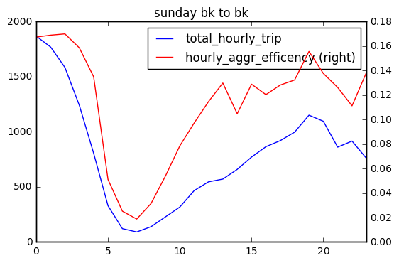
There are fewer trips from Brooklyn to Manhattan compared with trips within Brooklyn and the shared ride efficiency is quite low on Wednesday. On weekend, shared ride efficiency is above 0.06 only after 7 pm Sat to early Sunday. There is a peak on Sunday afternoon to Manhattan.

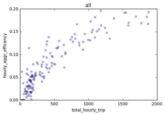
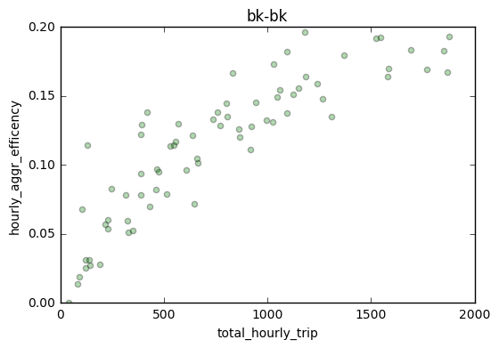
Linear Correlated?
To understand the correlation between total hourly trip and hourly shared efficiency, I first calculated the pearson correlation coefficient from 3 days (sat,sun,wed), 2 direcition (bk-bk, bk-man), and reported 0.899934, suggesting they are quite highly correlated. Again we can see there are fewer number of Brooklyn to Manhattan trips.

From the above analysis, I realize hourly shared ride efficiency is related to day of the week, hour of the day, destination (bk or man), as well as the total hourly trip. I then built a linear regression model to fit the data and try to predict a hourly shared ride efficiency of any given time.
def add_field(df,col1,col2):
    df['to'] = col1
    df['day'] = col2

# use numerical data to encode date and destination
add_field(sat_bk_bk_df,0,1)
add_field(sun_bk_bk_df,0,2)
add_field(wed_bk_bk_df,0,3)
add_field(sat_bk_man_df,1,1)
add_field(sun_bk_man_df,1,2)
add_field(wed_bk_man_df,1,3)
Sample size: 144 ( 3 days, 24 hour a day, 2 destination)
Features are ‘hour’, ‘to’, ‘day’
The label is ‘hourly_aggr_efficiency’
| hourly_aggr_efficiency | total_hourly_trip | hour | to | day | |
|---|---|---|---|---|---|
| 0 | 0.183372 | 1694 | 0 | 0 | 1 |
| 1 | 0.192233 | 1545 | 1 | 0 | 1 |
| 2 | 0.134911 | 1310 | 2 | 0 | 1 |
| 3 | 0.149407 | 1045 | 3 | 0 | 1 |
| … | … | … | … | … | … |
from sklearn.cross_validation import train_test_split
X_train, X_test, y_train, y_test = train_test_split(X,y,test_size=0.3, random_state=42)
reg = linear_model.LinearRegression()
reg.fit(X_train,y_train)
Using reg.score(X_test,y_test), I reported 0.82 R^2 score, suggesting a good fit of the data.
y_pred = cross_val_predict(reg, X_test, y_test,cv=5)

fig, ax = plt.subplots()
ax.scatter(y_test, y_pred,alpha=0.5)
ax.plot([y_test.min(), y_test.max()], [y_test.min(), y_test.max()], 'k--', lw=4)
ax.set_xlabel('Measured')
ax.set_ylabel('Predicted')
plt.show()
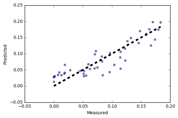
Last but not the least, I used cross validation to show the comparison of predicted value v.s. actual test value. As we can see, at lower shared ride efficiency, the predicted value seems to overestimate while as shared ride efficiency increase, the model seems to underestimate the value. Overall, the regression model provides us a rough idea about the shareability of Broolyn Trips.
References:
[1] L train service between Brooklyn and Manhattan to be shut down for 18 months starting in 2019, http://www.nydailynews.com/new-york/train-shut-18-months-starting-2019-article-1.2725118