In the previous post, I have discussed loss function in regression. In this post, I will elaborate how we develop loss function in classification when the output is discrete, rather than continuous.
This is No.5 post in the Connect the Dots series. See full table of contents.
In classification, the output \(y \) is discrete. With \(K\) classes, let’s label the class as \(1,2,…K\) and \(y \in \{1,2,…K\}\). For example, in binary classification, we can define \(label_1= 1, label_2 = 0\), or \(label_1= 1, label_2 = -1\), or \(label_1 = 100, label_2 = 200\), or \(label_1 = “red”, label_2 = “green” \). The actual value of each label does not matter, as they represent discrete and orderless categories. In the case of \(label_1=1, label_2 = 0\), although \(label_1 > label_2\) mathematically, the classification result is not affected if we switch their label values or use different label values.
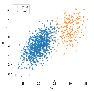
Conventionally, in binary classification, such as “disease v.s. healthy” and “target customer v.s. non-target customer” , we can use \(label_1=1\) to represent positive output and \(label_2 = 0\) to represent negative output, as shown in the figure above.
How can we find a good fitting function that returns discrete values?
Table of Contents
A simple and naive approach
In binary classification where \(y \in \{1,2\}\), we can try to simply treat the output as continuous \(y \in R\) as in linear regression, and find the linear regression coefficient \(\hat \beta\) using mean squared error:
\(\hat \beta= argmin_{\beta \in R^{p+1}} (y – \textbf{X} \beta) ^T(y – \textbf{X} \beta) \tag{1} \)
\(\hat \beta = ( \textbf{X}^T \textbf{X}) ^ {-1} \textbf{X}^Ty, \textbf{X} \in R^{N \times (p+1)} \tag{2} \)
Then we can define a decision boundary as a cut-off. For a given input \(x_i\), we can transform the expected continuous output \(x_i^T\hat \beta\) from linear regression to a discrete output as \(\hat f^{LS}(x_i) \) :
\(\hat f^{LS}(x_i) =\begin{cases}
1, & x_i^T \hat \beta <= boundary \\
2, & x_i^T \hat \beta > boundary \\
\end{cases} \tag{3} \)
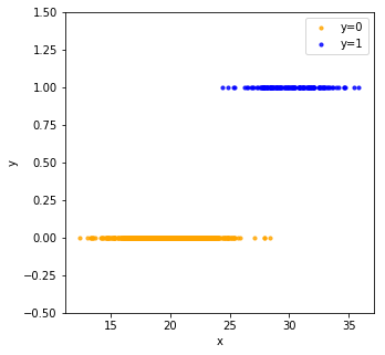
In the following example, we have a 1D input \(x\) and a binary output \(y \in \{0,1\}\)
Treating the output as continuous variable, we can fit the data with linear regression (red dashed line), and get the predicted \(y_{pred}\) for each \(x\).
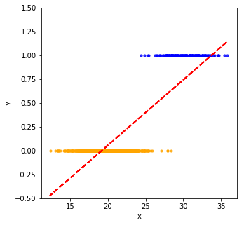
As shown in the following figure, the actual \(y_{train}\) takes discrete values 0 and 1, while the output from linear regression \(y_{predict}\) is continuous.

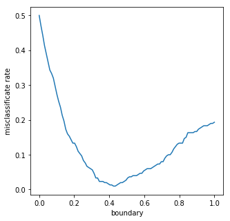
Using different decision boundaries, we can evaluate the total error on the data. We can use either mean squared error or misclassification error \(\sum_i^N I(y_{pred} \neq y_{real})\), which counts how many data points are misclassified. Because we have a 0-1 output here, mean squared error is equivalent to misclassification error.
As we can see, misclassification error reaches minimum when decision boundary is set as 0.44.
This decision boundary approach works well for binary classification. What if we have more than 2 classes? Since the discrete output does not have an intrinsic order, it is difficult to fit the data as linear regression directly.
Multiclass encoding with indicator variables
We can apply what we did for binary classification to multiclass if we can transform and encode multiclass as several binary classes. The idea is to use indicator variables (in feature engineering, it is often called one-hot encoding). For a \(K\) class problem with the output response \(G\), there are \(K\) indicators \(Y_k, k = 1,2,…K\) with
\(Y_k =\begin{cases}
1, & G=k \\
0, & else\\
\end{cases} \tag {4} \)
The overall indicator response matrix is \(Y = (Y_1, Y_2, …Y_K) \in R^{N \times K}\). For example, with \(N = 5, K = 3\), the indicator response matrix :
$$ Y = \begin{bmatrix}1 & 0 & 0 \\1 & 0 & 0 \\0 & 1& 0 \\0 & 1 & 0 \\0 & 0 & 1 \end{bmatrix} \in R^{5 \times 3} $$
For each column in \(Y\), we can fit a linear regression model to get the predicted continuous output as:
\(\hat Y = (\textbf{X}^T \textbf{X}) ^ {-1} \textbf{X}^TY \tag{5}\)
\(\textbf{X}\) is the model matrix with \(p+1\) columns with a leading columns of \(1\)’s for the intercept.
The coefficient matrix \(\hat {\textbf{B}} \in R^{(p+1) \times K}\) $ thus has \(K\) coefficients \(\hat \beta\) as in Equation 2.
To classify a new data \(x_i\), we can do the following:
- compute the fitted continuous output from each \(\hat \beta\) to get a \(K\) vector: \(\hat f(x_i)^T = (1, x_i^T)\hat {\textbf{B}} \tag {6.1} \)
- identify the largest component in the output and classify accordingly \(\hat G(x_i) = argmax_{k \in G} \hat f(x_i)_k \tag {6.2}\)
There is a serious problem with this regression approach for multiclass classification. Classes can be masked by others, which means there is no region in the feature space labeled as a certain class. Intuitively, this is caused by the rigid nature of the regression approach in Equation 6.2. Certain class \(k_*\) may never generate the maximum regression output. Data that should be classified as \(k_*\) will be misclassified as \(k_{max}\). Masking is not uncommon with large \(K\) and small \(p\). Examples can be found in reference [1] and [2].
To summarize what we have discussed so far, in binary classification, we can use the linear regression approach. In multiclass classification, the linear regression approach has its limitations, and we need to find alternative approaches.
Probability of classification
As discussed above, the problem of using linear regression for multiclass is caused by the rigid nature in Equation 6.2, in which we pick the class \(k\) with maximum \(\hat f\). We can modify this rigid 0-1 classification into a soft classification with \(\textbf{p}\) representing the probability of the data labeled as a given class.
Again, let’s start with binary class with the response \(G \in {1,2}\). Using Bayes rules, we can get the posterior probability given input \(x\).
\(p(G=1|X=x) \\ = \frac {p(G=1, X=x) } {p(G=1, X=x) + p(G=2, X=x) } \\ =\frac {1} { 1 + \frac {p(G=2, X=x)} {p(G=1, X=x) } } \\ = \frac {1} {1 + e^{-a} } = \sigma (a) \tag{7} \)
We define \(a\) as the natural log of the ratio \(\frac {p(G=1, X=x)} {p(G=2, X=x)} = \frac {p(G=1, X=x)} {1 – p(G=1, X=x)} \), which is also called odds in binary classification:
\(a = log \frac {p(G=1, X=x)} {p(G=2, X=x)} \tag{8}\)
\(a = log(odds) = log \frac {p} {1-p} \tag{9}\)
Equation 9 is called logit function which is the natural log odds.
The non-linear transformation function \(\sigma \) in Equation 7 is called logistic sigmoid function.
Sigmoid function is defined as:
\(\sigma (a) = \frac {1} {1 + e^{-a}} \tag{10}\)
and satisfies the symmetry property
\(\sigma(a) = 1 – \sigma(-a) \tag{11}\)
The derivative of the sigmoid function can be derived as following using the chain rule [3]:
\(\frac {\partial \sigma(a)} {\partial a} \\= \frac {\partial \frac {1}{1 + e^{-a}}}{\partial a} \\ = \frac {e^{-a}} {(1 + e^{-a})^2} \\ = \frac {1 + e^{-a} – 1} {(1 + e^{-a})^2} \\ = \frac {1 + e^{-a}} {(1 + e^{-a})^2} – (\frac {1} {1 + e^{-a}})^2 \\ = \frac {1} {1 + e^{-a}} – \sigma(a)^2 \\ = \sigma(a) – \sigma(a)^2 \\ = \sigma(a) (1- \sigma(a)) \tag{12}\)
The term “sigmoid” means S-shaped, and it squashes values in a continuous space \([- \infty, \infty ]\) into a finite interval \([0,1]\). Therefore, similar to the transformation in Equation 3, sigmoid function is a non-linear transformation from a continuous output to a finite output.
For a given input \(x_i \in R^{p+1}\), we can build a linear model with coefficients \(\beta \in R^{p+1} \).
\(a_i = x_i^T \beta = \beta^Tx_i \tag {13}\)
\(y_i = \sigma(a_i) = \sigma ( \beta^Tx_i) \tag{14} \)
\(x_i^T \beta \) is a scalar, thus \(x_i^T \beta =\beta^Tx_i \) . Note that we make assumptions of the linear format in Equation 13 as we did in linear regression. This is not to say the linear combination is the only representation.
Now let’s consider the loss function for Equation 14.
Loss function for classification
Can we use squared error?
Let’s start with the same error function as in linear regression:
\(L(\beta) = \sum_i^N(y_i – \hat y_i)^2 = \sum_i^N(y_i – \sigma( \beta^Tx_i))^2 \tag{15} \)
We could try to find \(\hat \beta\) to minimize \(L\) by setting its first derivative in Equation 16 as 0. The second derivative needs to be non-negative so that \(L\) is convex and the solution in the first derivative is global minimum.
\(L'(\beta) = \frac {\partial L}{\partial \beta} \\ = -2 \sum_i^N x_i \sigma( \beta^Tx_i) (1-\sigma( \beta^Tx_i)) (y_i – \sigma(\beta^Tx_i)) \tag{16} \)
\(L” (\beta) = \frac {\partial L’}{\partial \beta} = -2 \sum_i^N h_i \tag{17.1} \)
where \(h_i = [x_i^2\sigma( \beta^Tx_i)(1-\sigma( \beta^Tx_i))] [(y_i – 2(1+y_i)\sigma( \beta^Tx_i) + 3\sigma(\beta^Tx_i)^2)] \tag{17.2}\)
Now, we need to check if \(L” >=0\) (i.e. the loss function \(L\) is convex).
\(x_i, y_i\) can be viewed as constant. In Equation 17.2, the first element in the bracket the bracket \(x_i^2\sigma( \beta^Tx_i)(1-\sigma( \beta^Tx_i)) \) is always >=0, but the second element with \(y_i\) is not guaranteed to be non-negative. Therefore, mean squared error for logistic regression is not convex. This means that the solution for the first derivative as 0 is not guaranteed to be global minimum.
Can we use misclassification error?
I have shown that misclassification error can be used to find the optimal boundary in the linear regression approach. However, misclassification error is not differentiable, and we cannot use gradient-based approaches to find optimum.
Log-likelihood and maximum likelihood estimation (MLE)
You may have noticed that whenever people discuss logistic regression, MLE is always brought up as the fitting criterion. The idea is that we want to find a differentiable and convex loss function which allows us to solve the root of first-order derivative as the global optimum.
From Equation 14, we can see the probability/likelihood of a data \(p(G=k |X = x_i)\) can be defined as the sigmoid function:
\(p(x_i) = \sigma (a_i) = \sigma (\beta^Tx_i) \tag {18} \)
Thus the overall likelihood of all \(N\) observations can be written as the product of all probabilities:
\(\prod_i^N p(x_i|\beta) \tag{19} \)
Usually, we transform the product to its log format as a sum of log-likelihood. Note that the log here is natural log ln \(e^{log(x)} = x\)
The loss function can thus be defined as negative log-likelihood:
\(l(\beta) = -log(p(x_i |\beta)) \tag {20}\)
The total loss is
\(L(\beta) = -\sum_i^N log(p(x_i |\beta)) \tag{21}\)
In the simplest case when we have a binary response with \(y_i = 0\), when \(g_i = 1\) \(y_i = 1\) when \(g_i = 2\), and let \(p_1(x|\beta) = p(x|\beta) = \frac {1} {1 + e^{-\beta^Tx} }\), and \(p_2(x|\beta) = 1 – p(x|\beta)\).
\(L(\beta) \\ = -\sum_i^N \{ y_i log(p(x|\beta)) + (1-y_i) log(1 – p(x|\beta)) \} \\ = -\sum_i^N \{ y_i\beta^Tx_i – log(1 + e^{\beta^Tx_i }) \} \tag{22}\)
In order to minimize the loss function (i.e. maximize the log-likelihood), we set its first order derivative as 0:
\(L'(\beta) = \frac {\partial L}{\partial \beta} \\ = -\sum_i^N \{ y_i x_i – \frac {x_i e^{\beta^Tx_i}} {1 + e^{\beta^Tx_i }} \} \\ = -\sum_i^N \{x_i (y_i – p(x_i | \beta)) \} = 0 \tag{23}\)
The second order derivative:
\(L”(\beta) \\ = \frac {\partial^2L}{\partial \beta \partial \beta^T} \\ = \sum_i^N \{ x_i x_i^Tp(x_i | \beta) (1-p(x_i | \beta)) \} \tag{24} \)
Note \(x_i x_i^Tp(x_i | \beta) (1-p(x_i | \beta)) >=0 \). Thus the loss function \(L\) is twice differentiable and convex. We can then use the root of Equation 23 to get the global minimum value of \(L\).
Now we need to solve Equation 23 to get its root.
Newton method for convex optimization
Unlike linear regression in which the first derivative has a quadratic format and analytical solution, Equation 23 is nonlinear on \(\beta\) and does not have a closed-form solution. We need to use nonlinear optimization method, such as the Newton-Raphson method.
The intuition of the Newton-Raphson method is to approximate a function \(f\) using its derivative \(f'(x)\) in order to find the root \(f(x) = 0\), in an iterative manner:
\(x_{n+1} = x_n – \frac {f(x)} {f'(x)} \tag{25}\)
In the case of optimization, we need to solve the equation when first derivative is 0: \(f'(x) = 0\).
Thus we need to use the second derivative of f(x):
\(x_{n+1} = x_n – \frac {f'(x)} {f”(x)} \tag{26}\)
In the case of loss function \(L(\beta)\), we can iteratively compute \(\beta\)
\(\beta_{new} = \beta_{old} – (\frac {\partial^2 L}{\partial \beta \partial \beta^T}) ^{-1} {\frac{\partial L}{\partial \beta}} \tag {27}\)
As shown below, we can rewrite the second derivatives in a matrix format, \(X \in R^{N \times (p+1)}\), and \(\textbf{p} \) is the fitted probability with \(ith\) element \(p(x_i | \beta_{old} \), and \(W\) is a \(N \times N\) diagonal matrix with the \(ith\) diagonal element as \(p(x_i | \beta_{old}) (1-p(x_i | \beta_{old}))\)
\(\frac {\partial L}{\partial \beta} = – \textbf{X}^T(y – \textbf{p}) \tag{28}\)
\(\frac {\partial^2 L}{\partial \beta \partial \beta^T } =X^TWX \tag{29}\)
Thus we can write the Newton update as:
\(\beta_{new} \\ = \beta_{old} + (X^TWX)^{-1} \textbf{X}^T(y – \textbf{p}) \\= (X^TWX)^{-1}X^TW(X\beta_{old} + W^{-1}(y – \textbf{p})) \tag{30}\)
\(\beta_{new} = (X^TWX)^{-1}X^TWz \tag{31}\)
where \(z = X\beta_{old} + W^{-1}(y – \textbf{p}) \tag{32}\)
\(z\) is called adjusted response.
Recall in linear regression, we derive \(\hat \beta\) as $$\hat \beta = argmin_{\beta} (y – X\beta)^T(y – X\beta) = (\textbf{X}^T\textbf{X})^{-1}\textbf{X}^Ty $$
Equation 31 can be viewed as reweighted least square with \(W(\beta)\):
\(\beta_{new} = argmin_{\beta}(z – X\beta)^TW(z- X\beta) \tag{33} \)
We can solve Equation 30 in an iterative manner, an algorithm called iterative reweighted least square (IRLS).
What about gradient descent?
In practice, Logistic Regression is usually implemented using gradient descent. This is because the computation of the second derivative Hessian matrix (which is a \(p \times p\) matrix with \(p\) as the number of parameters to be optimized). Equation 30 includes matrix inversion which is computationally expensive. Therefore, from a computational perspective, at high dimension, Newton method is not prefered. At lower dimension, Newton method can converge to a global optimum much faster than gradient descent.
In addition, Newton method has a few limitations as discussed in [4]. 1) In 1D case, \(x_{n+1} = x_{n} – \frac {f(x_n)} {f'(x_n)}\), if \(f'(x_n) = 0\), i.e. \(x_n\) is a stationary point, the Newton update will not work. In multidimensional optimization case, if the eigenvalues of the Hessian matrix \(H\) are all positive as \(x\), a convex function \(f\) attains global minimum; if all eigenvalues are negative, \(f\) attains global maximum. However, if \(H\) has both positive and negative eigenvalues, \(f\) attains the minimax saddle point. 2) If there are more than one root for the function, choosing different starting point may converge to different roots. 3) If function \(f\) is reflected at its root \(x_*, f(x_*) = -f(-x_*)\), such as in \(f(x) = x^3 – 5x\), we could end up in a oscillating series \(x_{n+2} = x_n\) if we start with \(x_0 = 1\).
Gradient descent only needs to compute the first derivative, and updates parameters in the direction of the gradient. It is computationally cheaper than the Newton method. For a convex function, gradient descent could converge to global optimum, although it may also diverge from the optimum due to incorrect learning rate. For a non-convex function, gradient descent could converge to local optimum.
From sigmoid output to a discrete class
In binary classification, after we get \(\hat \beta\), we can predict \(\textbf{p}\) for given \(x_i\). \(\hat {\textbf{p}} \in [0,1]\) How can we then assign a single class based on \(\hat {\textbf{p}}\)? Intuitively, it seems 0.5 is a good decision boundary, since you get 50/50 head and tail for a fair coin flip. However, in practice, false positive may cost much more than false negative, and we may want to be very confident and only predict 1 when \(\hat {\textbf{p}}>0.9\), and vice versa.
Again, we can try different threshold boundaries as we did in the linear regression approach and evaluate which boundary performs the best. Here, boundary is a hyperparameter that needs to be tuned in the model evaluation process, which will be discussed in later posts.
Other discriminant classification methods such as support vector machine, tree-based classification, and perceptron in neural network, will be covered in later posts.
The other family of classification approach is called “generative approach” which makes a few assumptions of the joint distribution of the data. I will discuss the generative approach in later posts.
Take home message
There are 2 different approaches for classification: discriminant and generative. Linear logistic regression is a discriminant approach and uses sigmoid non-linear function to transform linear combinations of input to a probability. Logistic regression uses a different loss function from linear regression: log-likelihood, and uses an iterative approach to optimize.
Demo code can be found on my Github.
References
- https://www.quora.com/What-is-the-intuition-behind-the-masking-effects-on-linear-regression-in-multi-class-classification
- ESL-II 2nd Edition p105
- https://math.stackexchange.com/questions/78575/derivative-of-sigmoid-function-sigma-x-frac11e-x
- https://www.youtube.com/watch?v=K45mV2Mv-Ug
Hi Ju, do you have some background in numerical methods? I found it is very difficult for me to understand model-fitting through optimization at first. I started from the other end—write down the likelihood function or set up the model, then maximizing the likelihood function will naturally guide me to the territory of numerical optimization.
I think everyone has their own preferred way of learning. As long as it works for you, it is a good method. I also watched a lot of Youtube videos about optimization and found them very helpful.