In the previous post, I introduced Bayesian Optimization for black-box function optimization such as hyperparameter tuning. It is now time to look under the hood and understand how the magic happens.
This is No.12 post in the Connect the Dots series. See full table of contents.
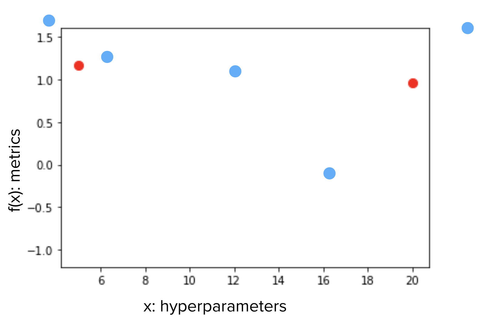
Let’s begin with an example. Say we have an input variable \(x\) and an objective metrics \(y=f(x)\). The function \(f(x) \) is a black box and all we know is for an input \(x\), we have a measurement \(y\). Now we have 2 measurements \(x_1, y_1\) and \(x_2, y_2\), and \(y_1 > y_2\), which \(x\) should we choose for the next measurement, in order to maximize \(f(x)\)?

If we assume the trend is linear, we may just draw a line across \(x_1, x_2\), and choose a point on the line, to the left of \(x_1\). But since we do not know if \(f\) is linear, we may want to stay in between the known range between \(x_1, x_2\), and closer to \(x_1\) (blue dots).
How do we decide whether we want to stay within the known range or go beyond? How close do we want to stay from \(x_1, x_2\)? And why do we decide (with mathematical rigor) to be closer to \(x_1\) than \(x_2\)?
When we are making decision about the next \(x\), we are using what we know to predict what is likely to be. Sounds familiar? Bayesian is coming.
As discussed in an earlier post, to better restrict the search space for fitting functions and to reduce computation cost, most of the time, we make some assumptions about the data and functions. The assumption in Bayesian Optimization is that it assumes the distribution of functions have a joint Gaussian distribution, in other words, it is a Gaussian Process.
Table of Contents
I. Gaussian process
A Gaussian Process defines a prior of the distribution of functions, and any finite number of these functions have a joint Gaussian distribution. The distribution of functions is usually unknown, but here, in order to make predictions, we assume it as a Gaussian Process.
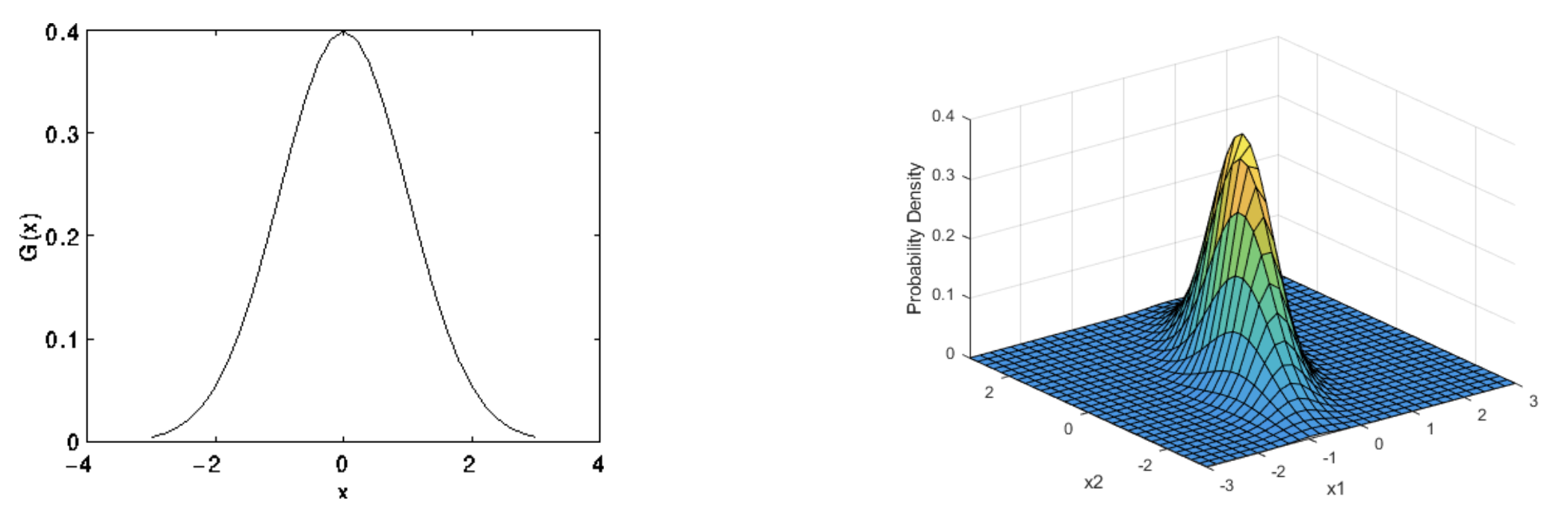
We are more familiar with Gaussian distribution of random variables. Shown in the diagrams below are 1D and 2D Gaussian [1,2]. Instead of describing the distribution of variables, Gaussian Process describes functions.
Similar to Gaussian distribution of variables, a Gaussian Process is also completely defined by its mean \(m(x)\) and covariance \(\sum\).
$$ m(x) = E[f(x)] \tag{1} $$
$$\sum = E[(f(x) – m(x))(f(x’) – m(x’))] \tag{2}$$
The covariance function of a Gaussian Process measures the similarity between input points to predict the function values. In the example before, we have intuitively selected a new point that is closer to the known point with higher value, with the assumption that closeness in input indicates closeness in output.
1. Kernel
This similarity measure can be represented as kernel:
$$\sum = K(x,x’) \tag{3}$$
You can think of kernel as feature map from low dimension to high dimension space \(\Phi(x): x \rightarrow R^x\).
\(\Phi(x) = K(.,x) \tag{4} \)
Instead of measuring the relationship between the output function in equation 2, we measure the relationship of the input mapped to a high dimenstion. One important property of kernel is “reproducing”:
\(K(x,x’) = <\Phi(x), \Phi(x’)> \tag{5} \)
\(<.,.>\) represents the inner product of 2 vectors.
2. Joint Gaussian
Any 2 functions \(f(x), f(x’)\) in a Gaussian Process can be written in a joint Gaussian:
$$\begin{bmatrix} f(x) \\
f(x’)\end{bmatrix}
\sim N
(\begin{bmatrix} \mu(x) \\ \mu(x’)\end{bmatrix},
\begin{bmatrix} K(x,x) & K(x,x’) \\ K(x’,x) & K(x’,x’) \end{bmatrix})
\tag{6}$$
The mean vector \(m\) is an \(n \times 1\) vector (which is always initiated as 0) and covariance matrix \(\sum\) is an \(n \times n\) matrix.
$$ m = \begin{bmatrix} \mu(x) \\ \mu(x’)\end{bmatrix} = 0 \tag{7}$$
$$ \sum =
\begin{bmatrix} K(x,x) & K(x,x’) \\ K(x’,x) & K(x’,x’) \end{bmatrix})\tag{8}$$
We can then represent a Gaussian Process by its mean and covariance
$$ f(x) \sim GP(m(x), K(x,x’)) \tag{9}$$
There are different types of covariance matrix \(K(x,x’)\). A commonly used one is squared exponential (SE), written as
$$ cov(f(x), f(x’)) = K(x,x’) = exp(-\frac{1}{2}|x – x’|^2) \tag{10}$$
Note that kernel is positive definite and the difference between \(x,x’\) is also non-negative.
3. From joint distribution to marginal distribution
Now that we have the joint distribution of \(f(x), f(x’)\) in equation 9, we can derive the marginal distribution of \(f(x’)\):
\(f(x’)|x,x’,f(x) \sim N(K(x’,x)K(x,x)^{-1}f(x), K(x’,x’) – K(x’,x)K(x,x)^{-1}K(x,x’)) \tag{11}\)
Let’s regard \(x, f(x)\) as known measurement from a Gaussian Process, and \(x’\) as unknown input in the same Gaussian Process. What we are doing in equation 11 is to compute the updated function distribution. The updated mean takes into account of the variance in the known data \(K(x,x)\), the distance between the unknown and known data \(K(x’,x)\), and the current known function value. The update covariance focuses only on the input, not function values.
Therefore, with equation 11, we can keep updating the Gaussian Process with more measurements.
II. Implement Gaussian Process
1. Compute covariance matrix
We can compute all kernel functions \(K\) in equation 11 directly, however, matrix inversion can be computationally expensive. Noticeably, the covariance matrix \(K\) is a symmetric and positive definite matrix, and thus as discussed in the matrix post before, we use Cholesky decomposition for \(K\).
$$K = LL^T \tag{12}$$
\(L\) is a lower triangular matrix and it is much easier to compute the inverse of a triangular matrix and there exist numerical solutions. The computation of \(L\) is numerically extremely stable and takes time \(\frac{n^3}{6}\), while the inverse of the original matrix \(K\) takes time \(n^3\).
Then the original matrix inverse is computed simply by multiplying the two inverses as:
$$K^{-1} = (LL^T)^{-1} = (L^{-1})^T(L^{-1}) \tag{13}$$
To solve a linear function:
$$Kx = b \tag{14.1}$$
write it as
$$LL^Tx = b \tag{14.2}$$
First solve
$$Ly = b \tag{14.3}$$
and by substitution
$$L^Tx = y \tag{14.4} $$
Thus, we can get \(x\) by solving equation 14.4..
Denote \(K\backslash b\) as solving a function \(Kx=b\), thus we can get \(x\) as
$$x = L^T\backslash(L\backslash b) \tag{15}$$
2. Compute marginal distribution
We first compute the Cholesky decomposition for \(K\).
$$L = cholesky(K(x,x) + \sigma^2_nI) \tag{16.1}$$
$$L_{ss} = cholesky(K(x’,x’) + \sigma^2_nI) \tag{16.2}$$
$$K(x,x’) = K(x’,x)^T \tag {16.3} $$
Note that we add a small identity matrix \(I\) for numerical reasons. This is because the eigenvalues of the matrix \(K\) can decay very rapidly and without stabilization the Cholesky decomposition fails. The effect is similar to adding additional independent noise of variance \(\sigma^2_n\).
In equation 11, we already have an expression for the mean and covariance of the marginal distribution of \(f(x’)\) with estimated mean:
$$ \bar{f(x’)} \\ = K(x’,x)(K(x,x) + \sigma^2_nI)^{-1}f(x) \\ =K(x,x’)^T(K(x,x) + \sigma^2_nI)^{-1}y \tag{17} $$
Define \(\alpha\) as
$$ \alpha = (K(x,x) + \sigma^2_nI)^{-1}y \tag{18}$$
Equivalent to equation 14.1, the coefficient matrix here is \((K(x,x) + \sigma^2_nI)\), which has the Cholesky decomposition as \(L\).
Thus solving equation, we have
$$\alpha = L^T\backslash (L\backslash y) \tag {19}$$
Thus equation 17 can be written as:
$$ \bar{f(x’)} \\ = K(x,x’)^T \alpha \\= L^T\backslash (L\backslash y) \tag {20}$$
We can then compute the variance of the prediction. Note that variance is the diagonal element in a covariance matrix.
From equation 11, we have the variance as:
$$V(f(x’) = K(x’,x’) – K(x’,x)K(x,x)^{-1}K(x,x’) \tag {21}$$
The second component can be written as
$$ K(x’,x)K(x,x)^{-1}K(x,x’) \\= K(x,x’)^T (LL^T)^{-1}K(x,x’) \\= (L^{-1} K(x,x’))^T (L^{-1}K(x,x’)) \tag {22}$$
Use
$$ v = L^{-1} K(x,x’) \tag {23.1} $$
Since \(K(x,x’) \) is a known matrix, we can easily compute \(v\) by solving
$$v = L \backslash K(x,x’) \tag{23.2}$$
Therefore,
$$V(f(x’)) = K(x’,x’) – v^Tv \tag {24}$$
In conclusion, we have the predicted mean and variance of the function \(f(x’)|x,x’,f(x)\) from equation 20 and 24.
3. Gaussian Process regression algorithm
Training data \(x,y=f(x)\), test data with unknown output \(x’\), covariance function \(K\), noise level \(\sigma_n^2\) [4].
1. \(L = choleskly(K(x,x),\sigma_n^2I)\)
2. solve \(\beta = L \backslash y\)
3. solve \(\alpha = L^T \backslash \beta\)
4. mean \(\bar{f(x’)} = K(x,x’)^T \alpha \)
5. solve \(v = L \backslash K(x,x’) \)
6. variance \(V(f(x’)) = K(x’,x’) – v^Tv\)
4. Generate samples from Gaussian Process
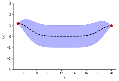
Once we have a Gaussian Process \(f(x) \sim GP(m, \sum)\), for each data \(x’_i \in x’\), we have a Gaussian distribution of the function value. In the diagram below, with a 1D input, for \(x’_i\), we have the mean function value (dashed line) \(\bar f(x’_i)\), and its variance \(\sum f(x’_i)\) (purple range). We can then generate sample \(u \sim N(0,I)\) using normal Gaussian generator for \(x’_i\).
III. Python implementation
See notebook [3] for details.
1) define kernel
def kernel(x1,x2,length_scale=1):
    sq_dist2 = np.sum(x1**2, 1).reshape(-1,1) + np.sum(x2**2, 1) - 2 * np.dot(x1,x2.T)
    return np.exp(- 1 * sq_dist2/ (2 * length_scale))
2) initiate with some known training data and unknown test data
Xtest = np.linspace(5,20,300).reshape(-1,1)
Xtrain = np.array([5, 20]).reshape(-1,1)
def f(Xtrain):# an unknown function
    return abs(np.exp(1/Xtrain) * np.sin(Xtrain))
ytrain = f(Xtrain)
3) compute all covariance matrix
length_scale = 3
sigma = 1e-6
K = kernel(Xtrain, Xtrain, length_scale)
K_s = kernel(Xtrain, Xtest, length_scale)
K_s_t = kernel(Xtest, Xtrain, length_scale) # transpose of K_s
K_ss = kernel(Xtest, Xtest, length_scale)
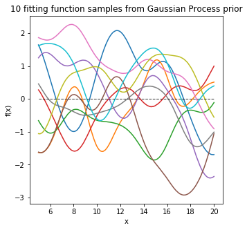
4) without training data, compute the prior function distribution
Use \(X_{test}\) with mean of 0 and covariance matrix of \(K_{ss}\)
L_ss = np.linalg.cholesky(K_ss + sigma *np.eye(len(Xtest)))
mean_prior = 0
f_prior = mean_prior + np.dot(L_ss, np.random.normal(size=(len(Xtest),10)))
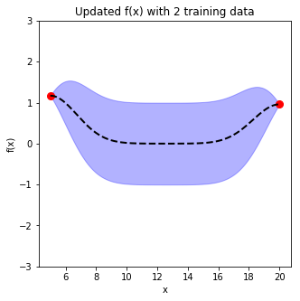
5) with training data, compute the marginal function distribution
Use the covariance matrix of \(X_{train}\), \(X_{test}\), and between \(X_{train}, X_{test}\) to compute the mean values of the function, and the standard deviation from the diagonal element in the covariance matrix in equation 11.
L = np.linalg.cholesky(K + sigma*np.eye(len(Xtrain)))
beta= np.linalg.solve(L,ytrain)
L_T = np.matrix.transpose(L)
alpha = np.linalg.solve(L_T, beta)
f_mean = np.dot(K_s_t, alpha)
v = np.linalg.solve(L, K_s)
f_V = np.diag(K_ss) - np.sum(v**2, axis=0)
f_stdv = np.sqrt(f_V)
6) length scale in the kernel function affects the estimate of function distribution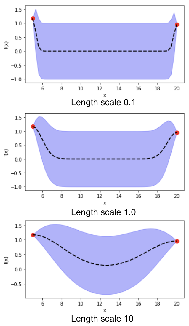
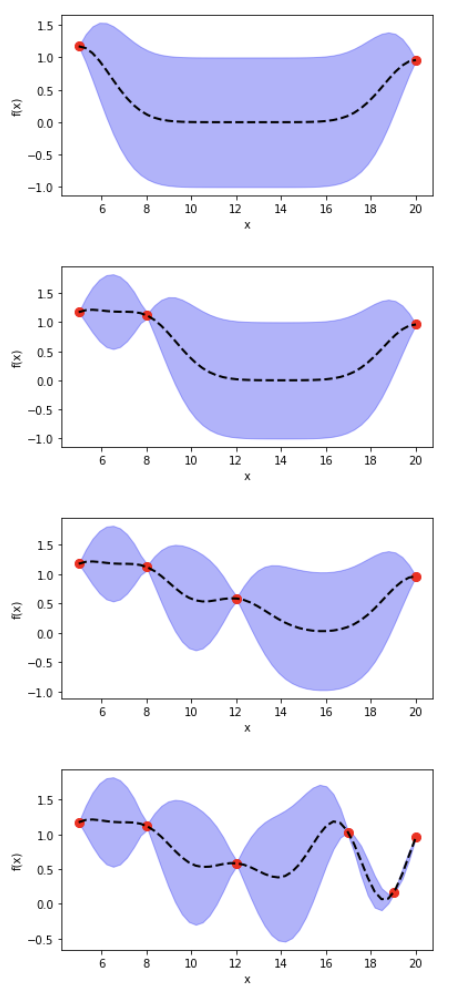
7) adding training data changes marginal function distribution, reducing variance
IV. Which point to choose next?
Having an updated Gaussian Process gives us an estimate of the function distribution, but it does not tell us directly which point to choose next. We need to define our own standard.
From equation 11, we have a predicted distribution of function \(f\) with its mean and variance. When we select the next point, we would like to choose a point that has higher function mean (exploitation) and higher variance (exploration). This exploitation-exploration tradeoff is similar to the one we face when choosing which song to listen to: do we listen to the song by our favorite artist, which we always like; or do we take a risk to try something new, which we may or may not enjoy?
Acquisition function
An acquisition function \(\alpha(x)\) captures the exploitation-exploration tradeoff. It is typically an inexpensive function to evaluate, and describes how desirable an input \(x\) in evaluating the black box function \(f\), say to minimize \(f(x)\). The problem now is to choose \(x\) that maximize \(\alpha(x)\) [5,6,7].
It seems we are just converting one optimization problem \(f(x)\) to another optimization problem \(\alpha(x)\), why are we doing this?
While \(f(x)\) can be expensive to evaluate (think of training and validating a complex neural net), \(\alpha(x)\) is much faster and cheaper to optimize.
As shown below, at each iteration \(t\), we select \(x\) that maximizes \(\alpha(x)\), the red triangle in the figure below [5].
\(x = argmax (\alpha(x)) \tag{25}\)

We can use different approaches to define the acquisition function.
1. Upper confidence bound (UCB)
The simplest acquisition function combines mean and standard deviation linearly for each point, with a parameter \(\beta\). \(\beta\) captures the degree of exploitation-exploration tradeoff: higher \(\beta\) means more exploration.
$$ \alpha(x) = \mu(x) + \beta \sigma(x) \tag{26}$$
2. Probability of improvement (PI)
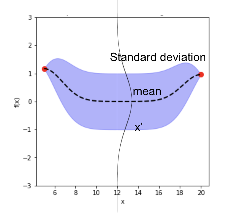
In PI acquisition function, we choose the next point based on the maximum probability of improvement (MPI) with respect to the current maximum. As shown in the figure below, for each unknown point \(x_1, x_2, x_3\), we have the function mean and standard deviation (depicted in a Gaussian bell curve vertically). We can easily compute the cumulative probability \(P(f(x) > c), c \in R\) in a Gaussian distribution.
The current maximum observed value is \(x^{+}\) with value \(f(x^{+})\). The area of the green shaded region gives the probability of improvement \(f(x_3) > f(x^{+}\)) at \(x_3\). The probability of improvement at \(x_1, x_2\) is negligible [5].

Probability improvement at any point \(x\) can be written as
$$ P(x) = P(f(x) > f(x^{+}) \tag {27} $$
With predicted mean \(\mu\) and standard deviation \(\sigma\), we have:
$$ P(x) = \Psi(\frac {\mu(x) – f(x^{+})}{\sigma(x)}) \tag {28} $$
\(\Psi\) is cumulative distribution function CDF.
3. Expected Improvement (EI)
As discussed above, PI takes into account the probability of improvement and not the magnitude of improvement for the next point. For example, \(x_1\) has 90% probability of 10% increase on \(\alpha(x)\), and \(x_2\) has 80% probability of 50% increase. PI would choose \(x_1\), but intuitively, we may want to consider \(x_2\) given its high magnitude of increase.
To quantify improvement over \(f\), we define
$$ I(x) = \max (0,f(x) – f(x^{+})) \tag{29}$$
Same as in equation 28, the current maximum observed value is \(x^{+}\) with value \(f(x^{+})\). \(f(x)\) represents the predicted function value at various \(x\).
The expected improvement (EI) can be evaluated analytically under the Gaussian Process model [6]:
\(EI(x) = \begin{cases} (\mu(x) – f(x^{+}) – \xi)\Psi(Z) + \sigma(x)\psi(Z) & , \sigma(x) > 0 \\ \max(0, \mu(x) – f(x^{+}) = 0 & , \sigma(x) = 0 \\ \end{cases} \tag {30}\)
\(Z = \frac {\mu(x) – f(x^{+}) – \xi}{\sigma(x)} \tag{31} \)
When \(\sigma(x) = 0\), this point has already be evaluated, and from equation 29, \(\mu(x) \leq f(x^{+}\), and thus \(\max(0, \mu(x)-f(x^{+}) = 0\).
When \(\sigma(x) > 0\), this point has not been evaluated. We rely on \(\Psi\) the cumulative distribution function CDF and \(\psi\) the probability density function PDF of the Gaussian Process to compute EI.
\(\xi\) in equation 30, like \(\beta\) in equation 26, captures the degree of exploration during optimization. Higher \(\xi\) means more exploration.
V. System optimization with Bayesian Optimizer
In practice, we are unlikely to implement Bayesian Optimization from scratch. There are packages we can use directly, such as scikit-optimize. One thing I like about scikit-optimize is that it provides Optimizer class, which has methods \(tell\) and \(ask\). \(tell\) loads previous history of \(x, f(x)\), and \(ask\) predicts the next point to evaluate.
This enables the application of Bayesian Optimizer as a separate step in a machine learning system. For example, we may have a complex multi-stage ML pipeline, various hyperparameters at each step, and convoluted metrics evaluation from different aggregated resources. The Bayesian Optimizer does not care about the details in system architecture. It only needs the historical output \(f(x)\), and input \(x\). While the Bayesian Optimizer here is a Python module, the ML pipeline can be in any language as long as it reads \(x\) – a set of all hyperparameters, and produces \(f(x)\) – such as AUCPR, as shown in the diagram below.

References
[1] 1D Gaussian https://homepages.inf.ed.ac.uk/rbf/HIPR2/gsmooth.htm
[2] 2D Gaussian https://www.mathworks.com/help/stats/multivariate-normal-distribution.html
[3] notebook https://github.com/yangju2011/Connect_the_Dots/blob/master/gaussian%20process/gaussian_process.ipynb
[4] Gaussian process https://katbailey.github.io/post/gaussian-processes-for-dummies/
[5] Eric Brochu, Vlad M. Cora and Nando de Freitas December 14, 2010 https://arxiv.org/pdf/1012.2599.pdf
[6] http://krasserm.github.io/2018/03/21/bayesian-optimization/
[7] https://www.cse.wustl.edu/~garnett/cse515t/spring_2015/files/lecture_notes/12.pdf
[8] https://cloud.google.com/blog/products/gcp/hyperparameter-tuning-cloud-machine-learning-engine-using-bayesian-optimization